Predicting Plant Growth Structures with Multimodal Data Using Convolutional Long Short-Term Memory (ConvLSTM)
By John Ivan Diaz
A multimodal deep learning model that predicts the next frame of plant growth by understanding two input modalities: growth patterns and environmental conditions. For instance, the model changes its prediction when the user adjusts pH level. Images of growth patterns pass through convolutional long short-term memory (ConvLSTM) layers, while environmental data passes through a series of layers such as time-distributed, reshape, and lambda. This produces two tensors with aligned temporal dimensions, which are concatenated to become a combined multimodal tensor. To generate the predicted frame, a 3D Convolution layer is employed.
In addition, a custom loss function is used to leverage the temporal dynamics and visual fidelity of Temporal Consistency and Mean Squared Error losses. The weighted sum of both is evaluated against each standalone loss quantitatively using metrics like Peak Signal-to-Noise Ratio (PSNR), Structural Similarity Index (SSIM), and Total Variation, and qualitatively through visual inspection. Results show that the custom loss delivers slightly better performance in preserving visual fidelity and temporal dynamics of slow-moving objects.
Within recent deep learning advancements, a convolutional long short-term memory (ConvLSTM) architecture exists that predicts future outcomes based on historical spatiotemporal data, such as images. It extends traditional LSTMs by replacing matrix multiplications with convolution operations, effectively handling spatiotemporal sequence prediction tasks. Other studies have utilized this architecture for tasks like weather forecasting and anomaly detection. They relied on established loss functions, such as Mean Squared Error (MSE), which focuses on pixel-level accuracy. Other established loss functions, like Temporal Consistency (TC), emphasize smooth temporal progression to avoid abrupt, unnatural transitions. However, these loss functions generally address only one aspect or strength at a time.
This project aims to develop:
A multimodal convolutional long short-term memory architecture capable of predicting future plant growth frames with respect to both past growth structures and environmental factors.
An improved loss function that unifies the attributes of Mean Squared Error and Temporal Consistency losses to capture pixel-level accuracy and temporal dependencies of plant growth frames during model training.
Development Phase
Data Pipeline Creation
Dataset
The dataset was split into three subsets: training, validation, and test sets. Conceptually, if one were to quickly view all images of a single sequence in succession, one would see the plant gradually growing over time. Formally, for the $s^{\text{th}}$ sequence, there is a set of frames:
where $I_{s,t}$ is an RGB image (at original resolution) of the plant on day $t$.
In addition to visual data, each sequence contains a CSV file holding parameters that describe environmental and growth conditions for each frame. Here, parameters include ambient temperature, soil moisture, luminosity, and soil pH. Thus, for each day $t$ in sequence $s$:
By pairing each image $I_{s,t}$ with its parameters $P_{s,t}$, the model receives a multimodal representation of plant growth, capturing both the visual appearance and the underlying conditions at each time step.
Image Rectification
Preprocessing is done to convert the raw data, initially stored as large RGB images and unscaled parameter values, into a format suitable for efficient model training. It involves image rectification, segmentation, resize, normalization, sequence length standardization, and augmentation.
Stereo images suffer lens distortion and misalignment between left and right views. Objects in both images must share identical scan-lines. Let $I_{s,t} \in \mathbb{R}^{H_0 \times W_0 \times 3}$ denote the RGB image captured on day $t$ of sequence $s$. Each image $I_{s,t}$ is rectified by a calibration map:
Each pair $(M_x^{(i,j)}, M_y^{(i,j)})$ stores the sub-pixel source coordinates in the distorted image that should be mapped to the rectified location $(i, j)$. The rectification operator is defined as:
The project isolated the plant from the background to focus the model's attention on the primary subject. To do this, a pre-trained YOLOv8 instance segmentation model is employed. Given an original image $I_{s,t}$, the segmentation model outputs a binary mask $M_{s,t}$ that highlights plant pixels only. The segmented image $\hat{I}_{s,t}$ is obtained via element-wise multiplication:
After segmentation, each image $\hat{I}_{s,t}$ is resized to a standardized dimension $(H,W)$ to reduce computational overhead and ensure a consistent input size:
The parameters in $P_{s,t}$ may differ widely in scale. To ensure that each parameter dimension contributes proportionately, global means $\mu_p$ and standard deviations $\sigma_p$ are computed across the training set. Each parameter vector is then normalized:
This yields zero-mean, unit-variance parameter distributions that allow the model to treat all parameters more uniformly.
Sequence Length Standardization
Since different sequences may have varying lengths $T_s$, a fixed sequence length $L$ is enforced. Here, $L = 45$ is used. If $T_s < L$, pre-padding is applied. The initial part of the sequence is padded with zero-valued frames and repeated initial parameter values to reach length $L$:
The project diversified the training data by applying random transformations to the input images during training. These transformations include horizontal flips or small rotations. If $\alpha$ is the probability of applying augmentation, each image $I_{s,t}^{\text{norm}}$ becomes $I_{s,t}^{\text{aug}}$ with probability $\alpha$. Here, $\alpha = 1$ is used.
Model Building
After all preprocessing steps, each sequence is represented as:
Images: $X_s = \{X_{s,1}, \ldots, X_{s,L}\}$, where each $X_{s,t}$ is the normalized (and augmented) image.
Parameters: $Q_s = \{Q_{s,1}, \ldots, Q_{s,L}\}$, where each $Q_{s,t} = P_{s,t}^{\text{norm}}$.
For one-step-ahead prediction, the first $L - 1$ frames and parameters are used as input, and the $L^{\text{th}}$ frame is the target. Thus:
In this manner of structuring data, the model learns to predict the next frame given a sequence of past frames and corresponding parameters.
Sequence Learning
To capture the temporal evolution of plant growth and the spatial structure of each frame, the project employed a Convolutional LSTM (ConvLSTM) architecture. It replaces the fully connected operations inside LSTM cells with convolutions that make it well-suited for spatial data. At each timestep $t$, the ConvLSTM updates its hidden and cell states $(H_t, C_t)$ based on the input $X_{s,t}^{\text{input}}$ and previous states $(H_{t-1}, C_{t-1})$:
Here, 2 ConvLSTM layers are employed. After processing the $L - 1$ input frames, a sequence of hidden states $\{H_1, \ldots, H_{L-1}\}$ is obtained that captures how the plant's appearance evolves over time.
Feedforward Mapping
In parallel, the parameter sequences $Q_{s,t}^{\text{input}}$ are passed through a time-distributed dense layer:
Each parameter vector is mapped into a feature embedding $Z_{s,t}$. This embedding is then broadcast (tiled) across the spatial dimensions $(H, W)$ to produce $Z_{s,t}^{\text{tile}}$.
Feature Fusion
By concatenating $Z_{s,t}^{\text{tile}}$ with the ConvLSTM output $H_t$, the model integrates both the visual and parametric modalities that allow the model to directly correlate changes in plant structure with environmental conditions:
where $\sigma$ is a sigmoid activation ensuring the predicted frame lies within $[0,1]$.
Deep Learning Structure
Deep learning structure. $t$ refers to time step, $temp$ refers to ambient temperature, $moist$ refers to soil moisture, $pH$ refers to pH level, $lum$ refers to luminosity.
Architecture Summary
Architecture summary.
Loss Function
To guide the training process, the loss function measures discrepancy between predicted frames $\hat{X}_{s,L}$ and the ground truth $X_{s,L}$. First, Mean Squared Error (MSE) loss encourages pixel-level accuracy by penalizing large deviations between predicted and true pixel values:
where $N = H \times W \times 3$, and $\hat{x}_i$ and $x_i$ denote the ground-truth and predicted intensity values for pixel $i$.
Second, consider a sequence of frames $\{X_1,X_2,\ldots,X_T\}$ and their predictions $\{\hat{X}_1,\hat{X}_2,\ldots,\hat{X}_T\}$. Let $\Delta X_t = X_t - X_{t-1}$ represent the frame-to-frame change in the ground-truth, and $\Delta\hat{X}_t = \hat{X}_t - \hat{X}_{t-1}$ the corresponding change in the predictions. Temporal Consistency (TC) loss preserves temporal dynamics by enforcing that predicted differences resemble real differences:
The project blended MSE and TC. By assigning weights $\alpha$ and $\beta$ to the MSE and TC terms, respectively, the unified loss seeks a balanced optimization path:
Here, $\alpha = 1.0$ and $\beta = 0.2$ is used. Adam optimizer is applied to minimize the chosen loss, iterating over batches of sequences to adjust model parameters.
Model Evaluation
Evaluation Metrics
The model is evaluated under three training scenarios: using only MSE loss, only temporal consistency (TC) loss, and the unified loss. For each scenario, assessment is done by comparing the predicted frames $\hat{X}$ with the ground-truth frames $X$. The metrics employed are:
Mean Squared Error (MSE)
Peak Signal-to-Noise Ratio (PSNR)
Structural Similarity Index Measure (SSIM)
Temporal Consistency (TC)
Total Variation (TV)
Visual inspection
MSE computes the average squared difference between ground-truth pixel intensities $x_i$ and predicted pixel intensities $\hat{x}_i$ over $N$ pixels, as shown in the equation below. Lower MSE values approaching 0 suggest better pixel-level correspondence.
PSNR indicates how perceptually clean and less distorted the image is by transforming MSE into a decibel scale as shown in the equation below. Higher PSNR values within 40-50 dB suggest lesser noise.
SSIM examines luminance, contrast, and structural details by examining mean intensities $\mu_x$, $\mu_{\hat{x}}$, variances $\sigma_x^2$, $\sigma_{\hat{x}}^2$, and covariance $\sigma_{x\hat{x}}$, as shown in the equation below. SSIM values approaching 1 suggest preservation of perceptual quality.
TC evaluates whether the predicted sequence follows the real temporal progression of plant growth without abrupt or unnatural transitions by comparing differences $\Delta x_{t,i}$ and $\Delta\hat{x}_{t,i}$ of pixel intensities at pixel $i$ between consecutive frames $t$, as shown in the equation below. Lower TC values approaching 0 suggest that predicted temporal changes closely match actual temporal changes.
TV evaluates the degree of local intensity fluctuations across the image by summing the absolute intensity gradients between neighboring pixels $(h,w)$, where $\hat{x}_{h,w}$ refers to the predicted intensity at row $h$ and column $w$, and the summations run over valid neighboring pixel coordinates, as shown in the equation below. Lower TV values suggest smoother spatial distributions and fewer artifacts.
Lastly, visual inspection assesses images based on subjective, human-based assessment.
Model Training and Evaluation Flowchart
Model training and evaluation flowchart.
Training Loss Curves
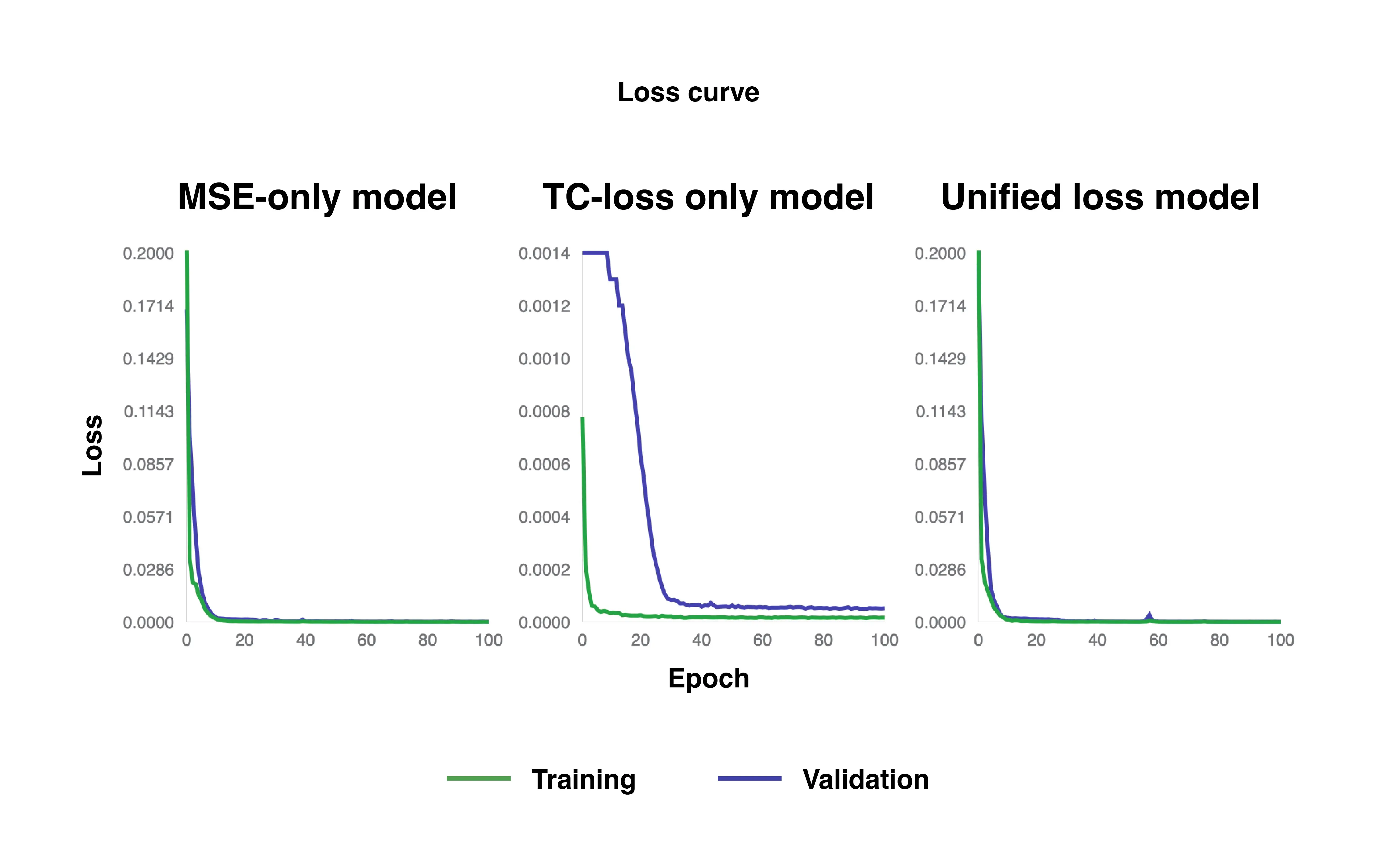
Loss curves of MSE-only loss, TC-only loss, and unified loss models.
For all three scenarios, the losses consistently decrease, as shown in the figure above, which is a positive sign that the model is effectively learning to predict subsequent frames of plant growth structures. However, around 20 epochs, all models begin to converge. This suggests that the dataset, or the plant growth structures it represents, is relatively straightforward for the model to learn. Such an outcome is somewhat expected due to the segmentation process, where only the plant regions are retained and all non-plant elements are removed which reduced complexity. However, this also indicates that the dataset is limited and lacks diversity in terms of plant growth structures which is not providing more complex scenarios for the model to further improve upon.
Training Metric Curves
MSE curves of MSE-only loss, TC-only loss, and unified loss models.
Looking at MSE curves shown in the figure above, both the MSE-only loss and unified loss models achieve good pixel-level accuracy by converging at around 20 epochs for both training and validation. In contrast, the TC-only loss model does not fully converge even after 100 epochs. However, throughout the epochs, the MSE metric for the TC-only model gradually decreases which indicate a steady yet slow improvement in pixel-level accuracy. It reflects the inherent nature of the TC loss, which prioritizes maintaining realistic temporal progressions of plant growth without abrupt transitions rather than directly optimizing for visual fidelity.
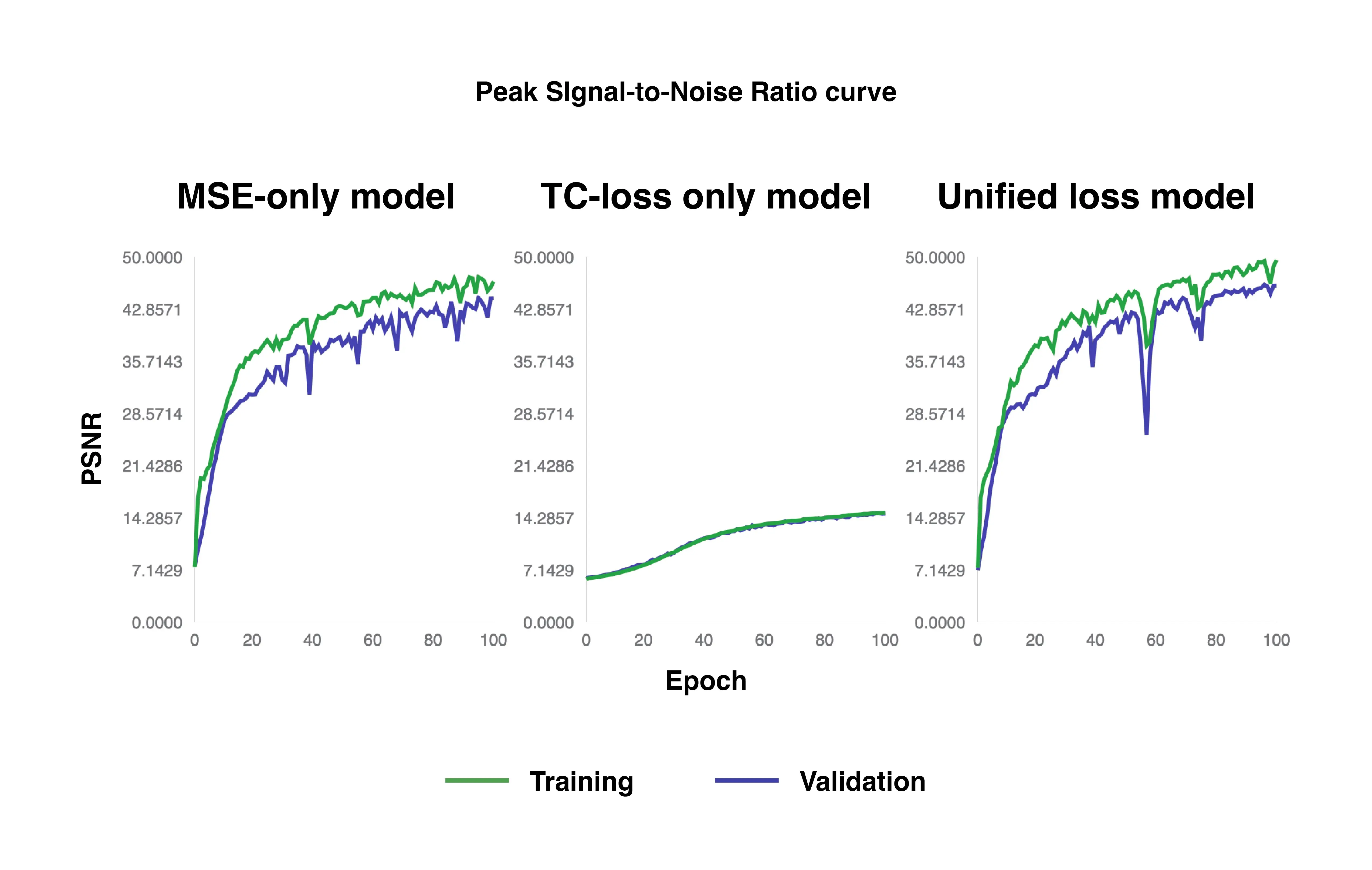
PSNR curves of MSE-only loss, TC-only loss, and unified loss models.
The same applies to PSNR, SSIM, and TV metrics. The MSE-only loss and unified loss models quickly achieve lower noise, better perceptual quality preservation, and fewer artifacts compared to the TC-only loss model.
The MSE-only loss model reaches the good benchmark of around 40 dB at approximately 30 epochs for the training set and 55 epochs for the validation set for PSNR. The unified loss model is slightly faster, achieving this level at about 25 epochs for the training set and 35 epochs for the validation set. In comparison, the TC-only loss model performs substantially worse, never reaching 40 dB and only achieving about 15 dB for both training and validation throughout the entire 100 epochs.
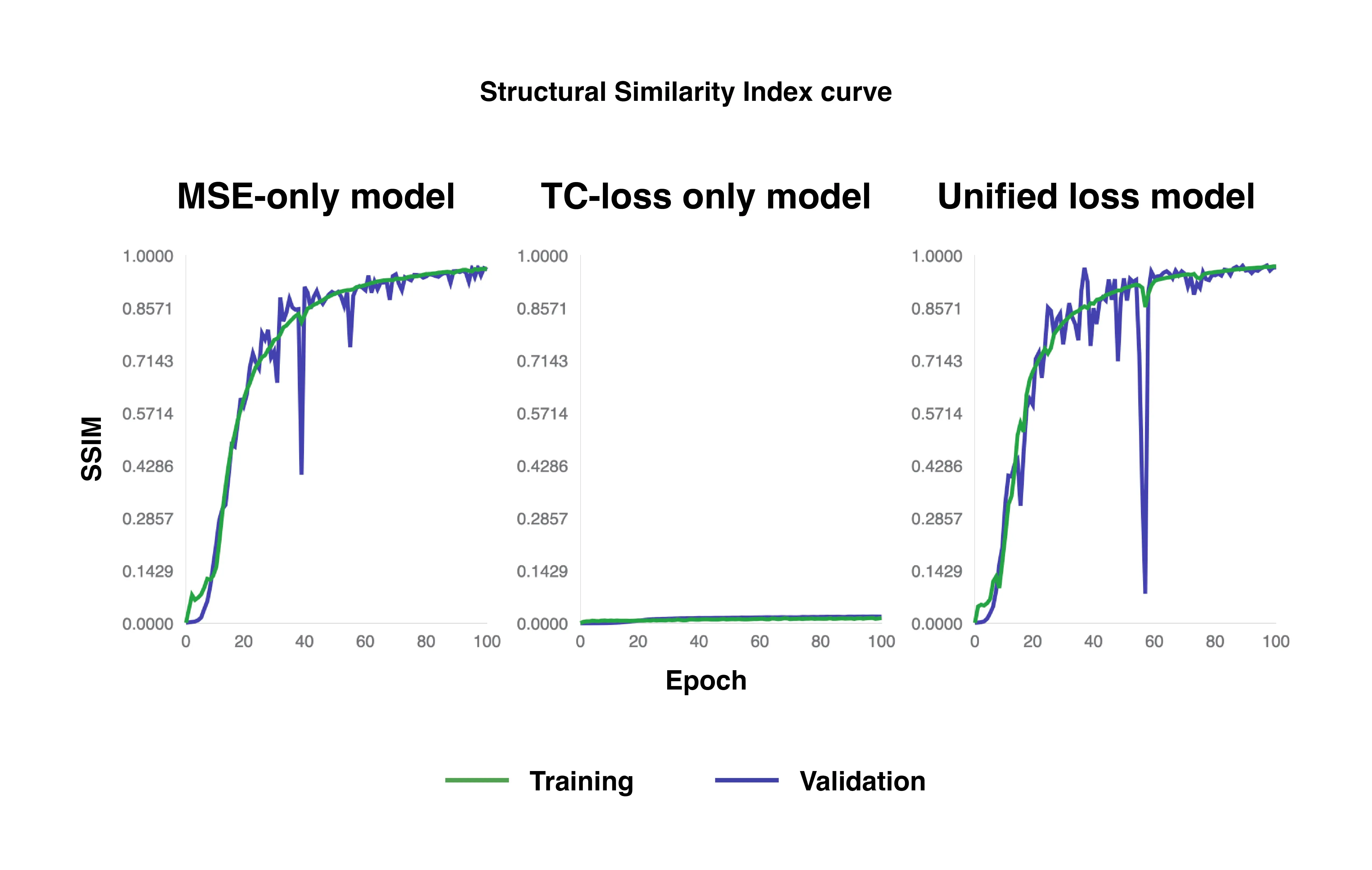
SSIM curves of MSE-only loss, TC-only loss, and unified loss models.
Both the MSE-only loss and unified loss models reach a good benchmark of 0.9 or higher at roughly 50 epochs for both training and validation sets for SSIM. However, the TC-only loss model remains far from this target, only reaching about 0.015 and 0.020 for training and validation, respectively, over the entire 100 epochs.
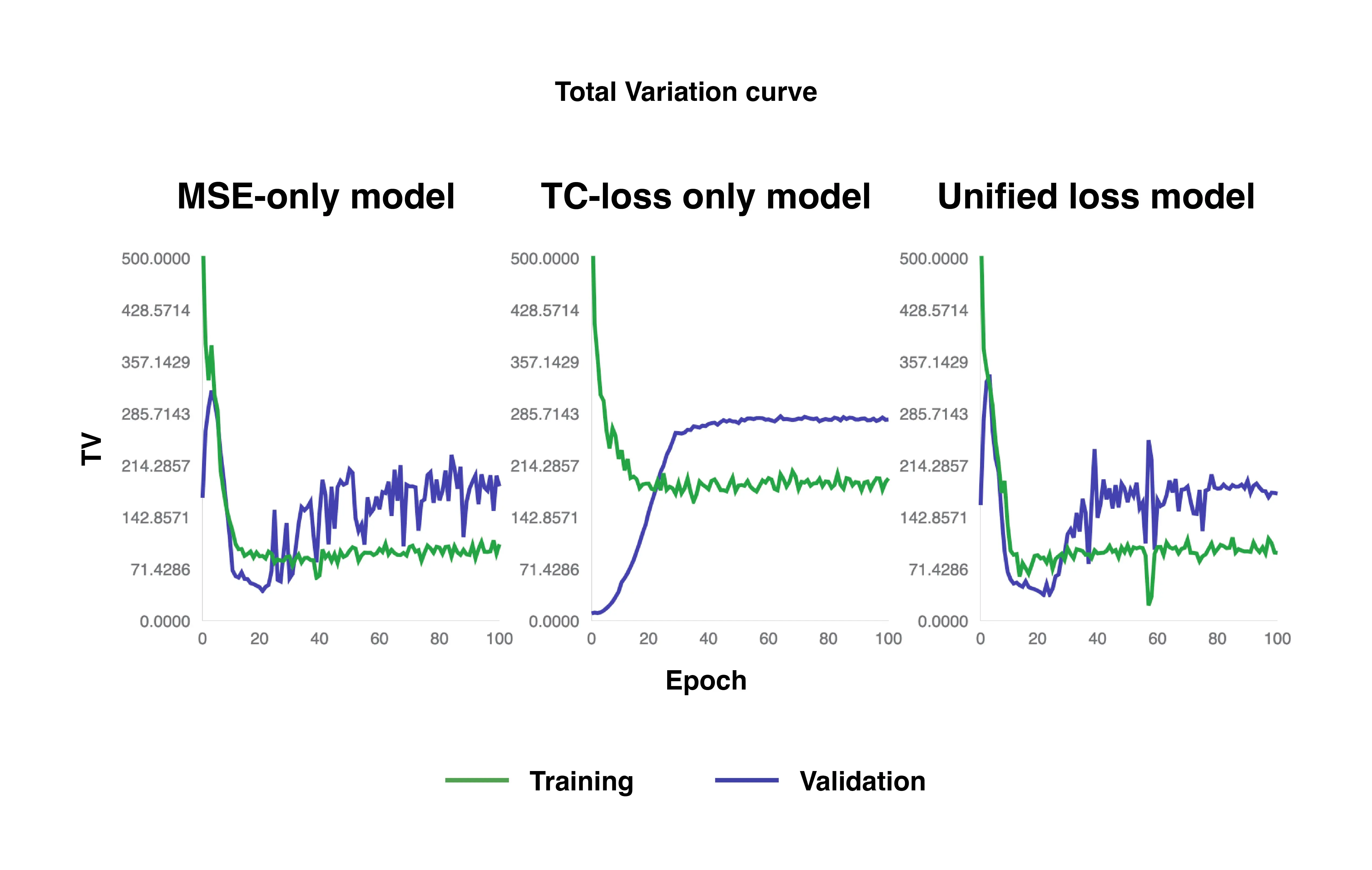
TV curves of MSE-only loss, TC-only loss, and unified loss models.
Both the MSE-only loss and unified loss models converge to approximately 100 at around 20 epochs for the training set, and about 200 at around 40 epochs for the validation set for TV. While the TC-only loss also minimizes TV and converges at around 20 epochs for training and 40 epochs for validation, its minimum TV values are slightly higher, at about 200 for the training set and 300 for the validation set.
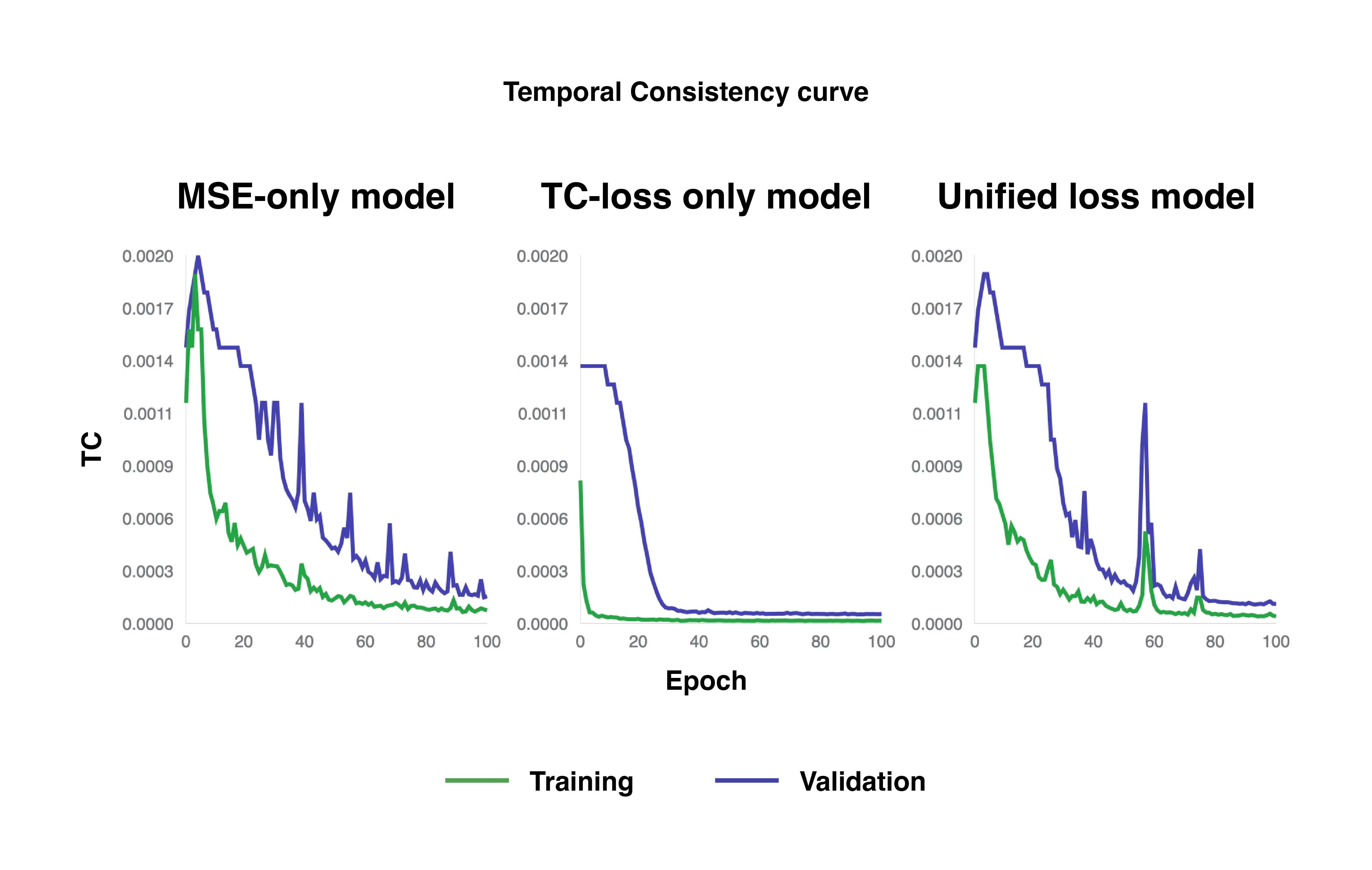
TC curves of MSE-only loss, TC-only loss, and unified loss models.
Meanwhile, with TC, the TC-only loss model demonstrates its strength of maintaining temporal progression without abrupt transitions, converging near 0 at about 10 epochs for the training set and 30 epochs for the validation set. In comparison, the MSE-only loss and unified loss models converge near 0 much later, at around 80 epochs for both training and validation sets.
Quantitative Testing Results
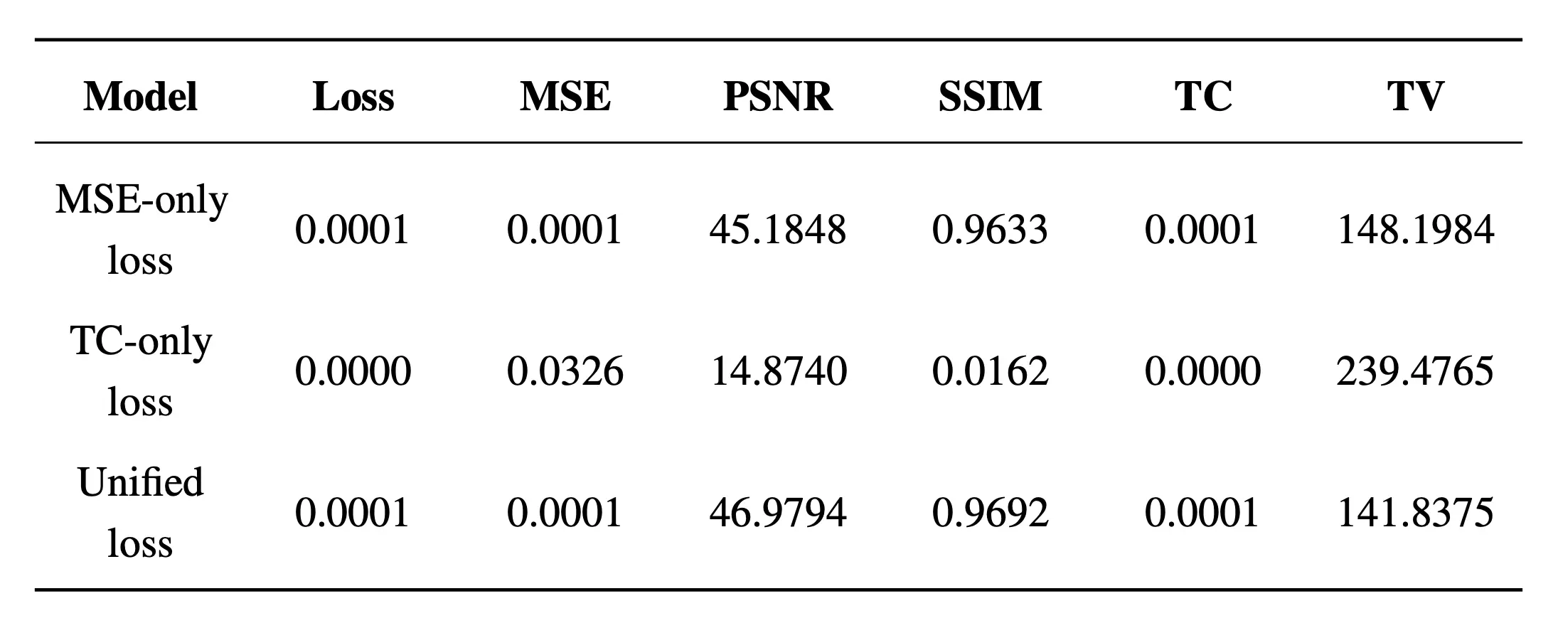
Evaluation results of MSE-only loss, TC-only loss, and unified loss models.
Table 5.2 shows results of the model evaluated on the test set, which the model did not see during training. The model using TC-only loss shows poorer results in terms of visual fidelity. Its PSNR of 14.8740 and SSIM of 0.0162 are both far below the good result benchmarks for cleaner and perceptually preserved quality. Its MSE and TV of 0.0326 and 239.4765, respectively, are also higher (worse) than those of the MSE-only loss and unified loss models. However, the TC-only model excels in the TC metric, scoring 0, which reflects a temporal progression free from abrupt transitions.
The models using MSE-only loss and unified loss yield similar results that meet the benchmarks for good performance across all metrics. The unified loss model, however, demonstrates slightly better outcomes, with a higher (better) PSNR of 46.9794 compared to the MSE-only loss model's 45.1848, a higher (better) SSIM of 0.9692 versus the MSE-only loss model's 0.9633, and a lower (better) TV of 141.8375 compared to the MSE-only loss model's 148.1984. These findings indicate less noise, more preserved perceptual quality, and fewer artifacts. Both models achieve similarly low MSE and TC values of approximately 0.0001, although neither reaches a flat zero TC value as the TC-only loss model does, reaffirming the TC-only model's strength in ensuring smoother temporal progression.
Qualitative Testing Results
The project used dataset consisting plant growth sequences captured under consistent environmental parameter values. Consequently, it cannot evaluate scenarios where parameter values vary. During model testing, the same parameter values from the dataset are used for rendering predicted images, with an ambient temperature of 25°C, soil moisture at 50%, luminosity at 700 lux, and soil pH at 7.5. The window size for generating each predicted frame is 30, and at every future time step, the window moves forward by one stride.
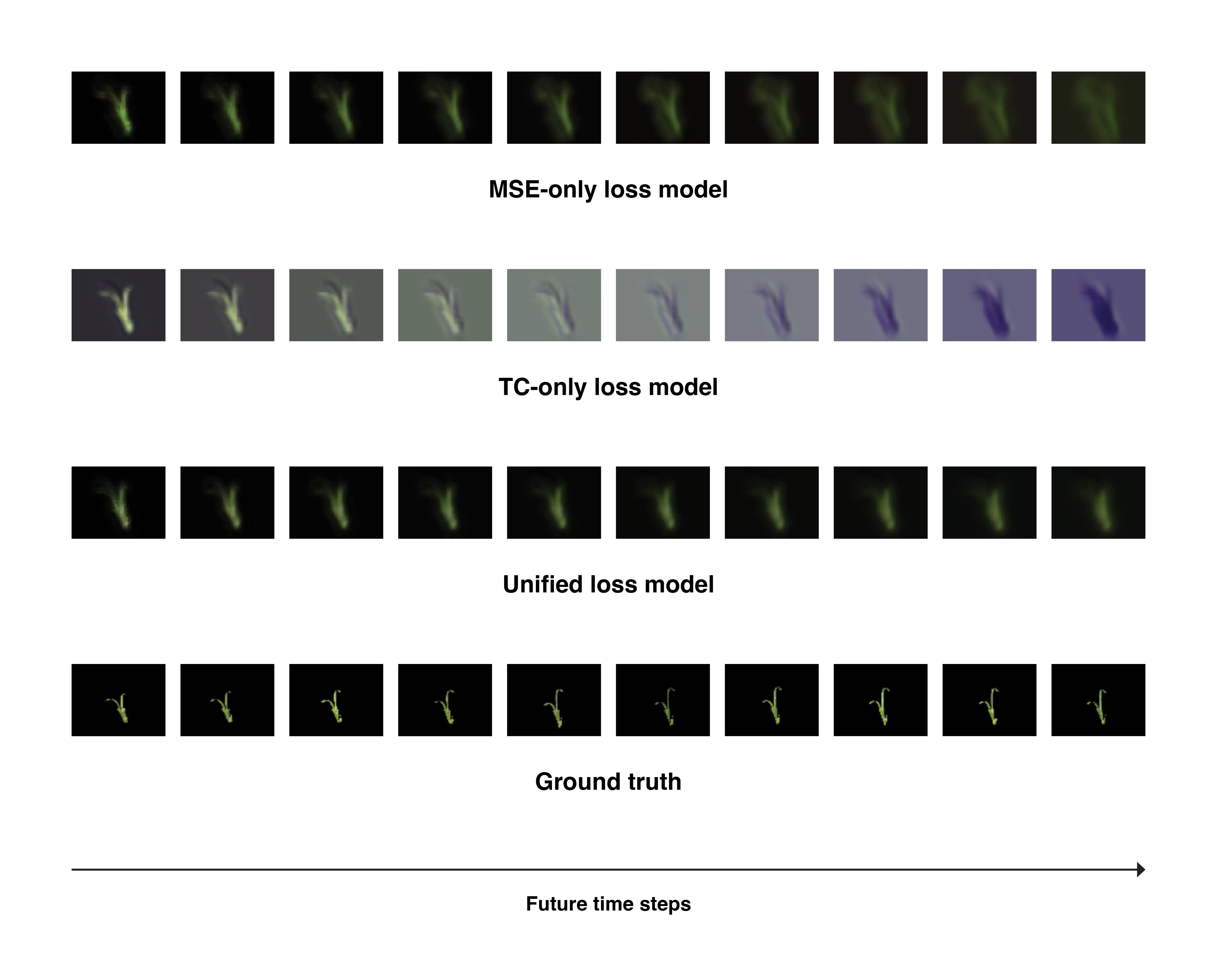
Rendering prediction images at 10 future time steps from MSE-only loss, TC-only loss, and unified loss models.
Rendering predicted images from all models, as shown in the figure above, demonstrates where the unified loss function stands out. Visually, at just one time step ahead, all scenarios still represent the plant's form, although with the TC-only loss model, the plant's color appears somewhat washed out, and the background no longer remains pitch-black as in previous frames. After predicting 10 time steps ahead, the TC-only loss model's plant appearance disappears, and the background strays even further from black, although a faint contour remains that reflect the temporal progression without abrupt transitions. In the MSE-only loss model, the plant's color persists, but its form becomes increasingly blurred and distorted over extended time steps, and by the 10th predicted frame, the background is subtly turning gray. In comparison, the unified loss model retains the plant's color and a more identifiable shape over the same period, while the background remains pitch-black up to the 10th predicted image. However, it still exhibits increasing blurriness as predictions extend further into the future.