By John Ivan Diaz
A deep learning model trained to classify CIFAR-100 images of reptiles into five categories: crocodile, dinosaur, lizard, snake, and turtle. It uses convolutional, pooling, and fully connected layers, along with techniques such as data augmentation, dropout, and early stopping. The model achieved decent accuracy despite the challenge of limited training images.
Discovery Phase
Use Case Definition
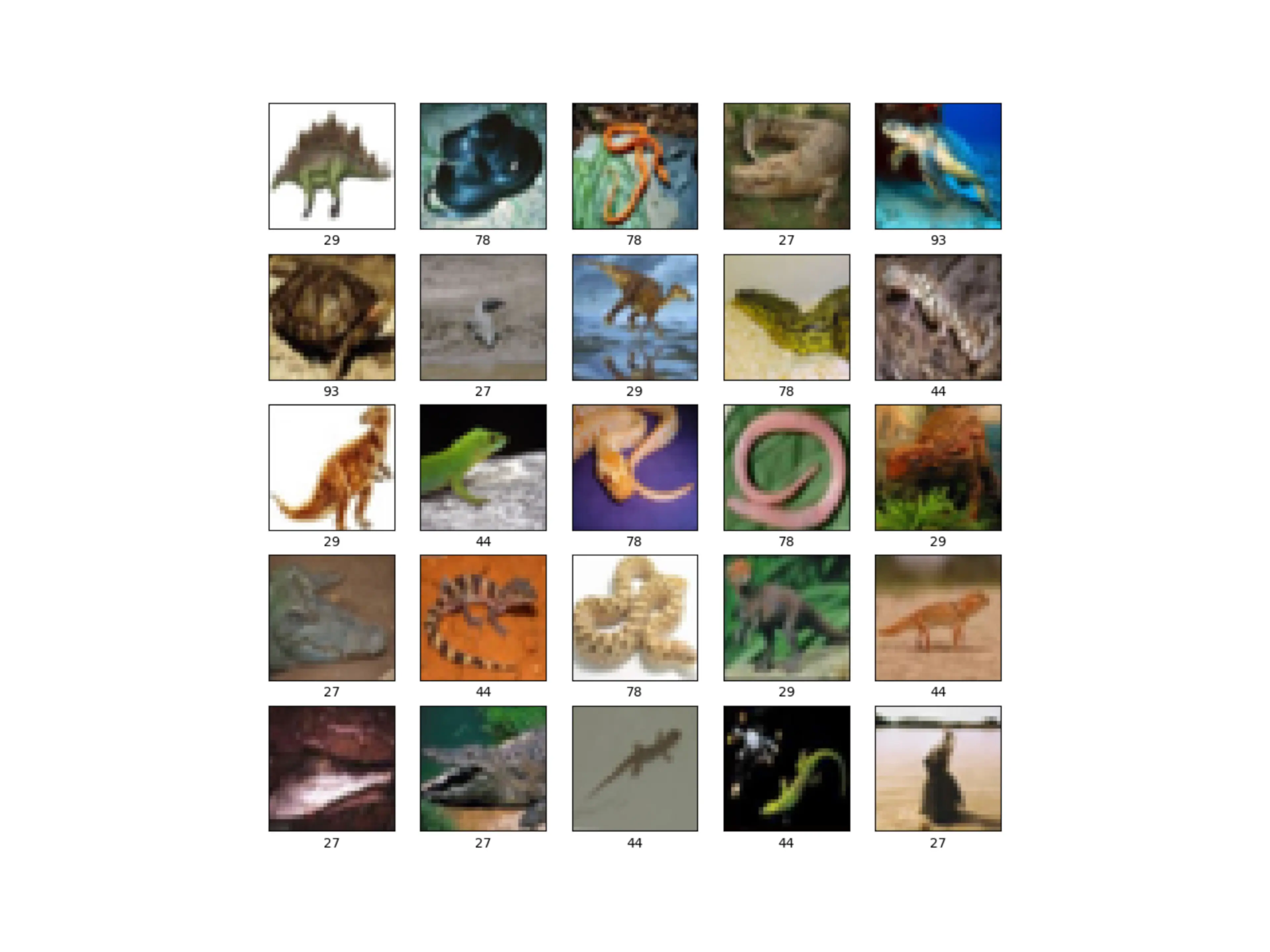
This project solves an image classification problem using the CIFAR-100 dataset, specifically within the “Reptiles” superclass. The project is tasked with developing a deep learning model capable of discerning the type of reptile depicted in an image. The “Reptiles” superclass comprises five subclasses, representing the target labels the model will learn to recognize through training.
Considering the project has labeled data indicating the correct classification for each image, the approach is rooted in Supervised Learning. Furthermore, the task at hand is Classification, as the labels are categorical (e.g., crocodile, lizard, etc.), as opposed to Regression, which deals with continuous outputs.
Data Exploration
In this phase, the project focuses on acquiring the data necessary to train and evaluate the deep learning model. Specifically, the project will utilize the “Reptiles” superclass from the CIFAR-100 dataset for this purpose.
Upon inspecting the CIFAR-100 dataset dictionary, which contains 20 superclasses, this project will only focus on one superclass, “Reptiles”. “Reptiles” is the 16th superclass in the list, but since indexing starts from 0, it is indexed at 15. Hence, the project states REPTILES_INDEX = 15 in the code.
Furthermore, the project converted the index lists to NumPy arrays before extracting the “Reptiles” images and labels. This step enables the project to quickly select the specific images of the superclass that are needed and to work efficiently with the tools that assist in building and training the machine learning model.
Architecture and Algorithm Selection
Given that image classification problems are being addressed, the project relies on deep neural network architectures that are specifically designed for processing, analyzing, and making predictions from visual data. Among the various architectures available, Convolutional Neural Networks (CNNs) are recognized as the most effective and widely adopted solution for tasks related to images. CNNs excel at identifying patterns within images, such as edges, textures, and shapes, thanks to their unique structure that emulates the way the human visual cortex interprets visual information.
The architecture comprises several layers, each contributing cumulatively towards the goal of classifying images, as illustrated below:
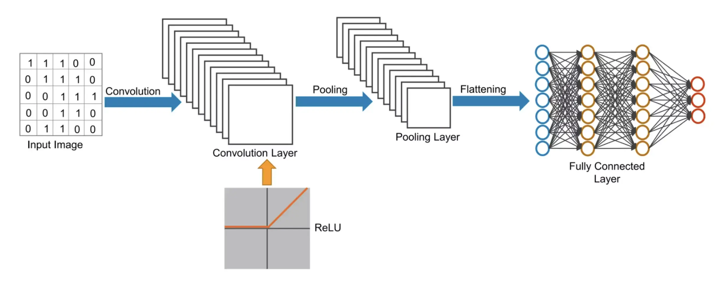
Each component plays a vital role in the capability of a Convolutional Neural Network (CNN) to classify images. The Convolution Layers are responsible for extracting and activating relevant features. Pooling Layers reduce dimensionality and highlight the most significant features. Finally, Fully Connected Layers make the ultimate classification decisions based on these features.
Development Phase
Data Pipeline Creation
Data Splitting
The CIFAR-100 dataset provides a set of training and test images. Within the “Reptiles” superclass, each of the five subclasses includes 500 training images and 100 test images. This totals 3,000 images for the “Reptiles” superclass, with 2,500 dedicated to training and 500 set aside for testing.
The project further divided the data from the “Reptiles” superclass into three distinct sets: Training Set, Validation Set, and Test Set. This division serves multiple purposes:
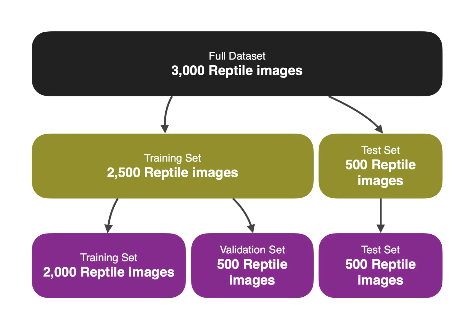
The Training Set is used to fit the model, allowing it to learn and recognize patterns. The Validation Set is utilized not for training but for tuning hyperparameters. It provides an unbiased evaluation of the model fit during the training phase. The Test Set offers an unbiased evaluation of the final model fit and is only employed once the model is fully trained.
Given that the CIFAR-100 dataset already segregates data into Training and Test Sets, the project derived the Validation Set by allocating a percentage of the Training Set for this purpose. For the model, the project allocated a Test Size of 0.2 or 20% of the 2,500 training images to form the Validation Set. This means the Validation Set comprises 500 images, matching the size of the Test Set, which already contains 500 images.
By partitioning the dataset in this manner, a rigorous evaluation framework is established. It allows the model to be trained on one data subset, fine-tuned with another, and ultimately tested on unseen data. This approach ensures that the model’s performance is not only effective on known instances but also generalizable to new data.
Feature Encoding
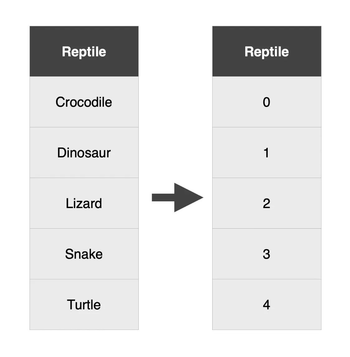
The dataset encompasses five labels corresponding to the subclasses within the “Reptiles” superclass. To effectively utilize these categorical text labels for model training, they must be transformed into numerical values. This transformation is achieved through feature encoding.
While various feature encoding methods exist, the project has opted for Label Encoding, wherein each unique category label is assigned a distinct integer.
Normalization
Working with images entails dealing with pixel values that range from 0 to 255. Normalizing these values to fall between 0 and 1 aids the model’s efficiency in understanding and processing the images. By scaling down the pixel values, a ‘common ground’ for all images is created. This process is crucial as it enables the model to learn patterns and make predictions more quickly and accurately by mitigating potential confusion caused by the wide variations in pixel value magnitudes. Normalization is especially beneficial for the deep neural network architecture that will be used, which will be discussed in subsequent phases.
Model Building
Convolution Layer
The Convolution Layer is the foundational building block of the CNN model. It executes a mathematical operation known as convolution. This layer utilizes filters (or kernels) that move across the input image (or the output from the preceding layer), producing feature maps in the process.
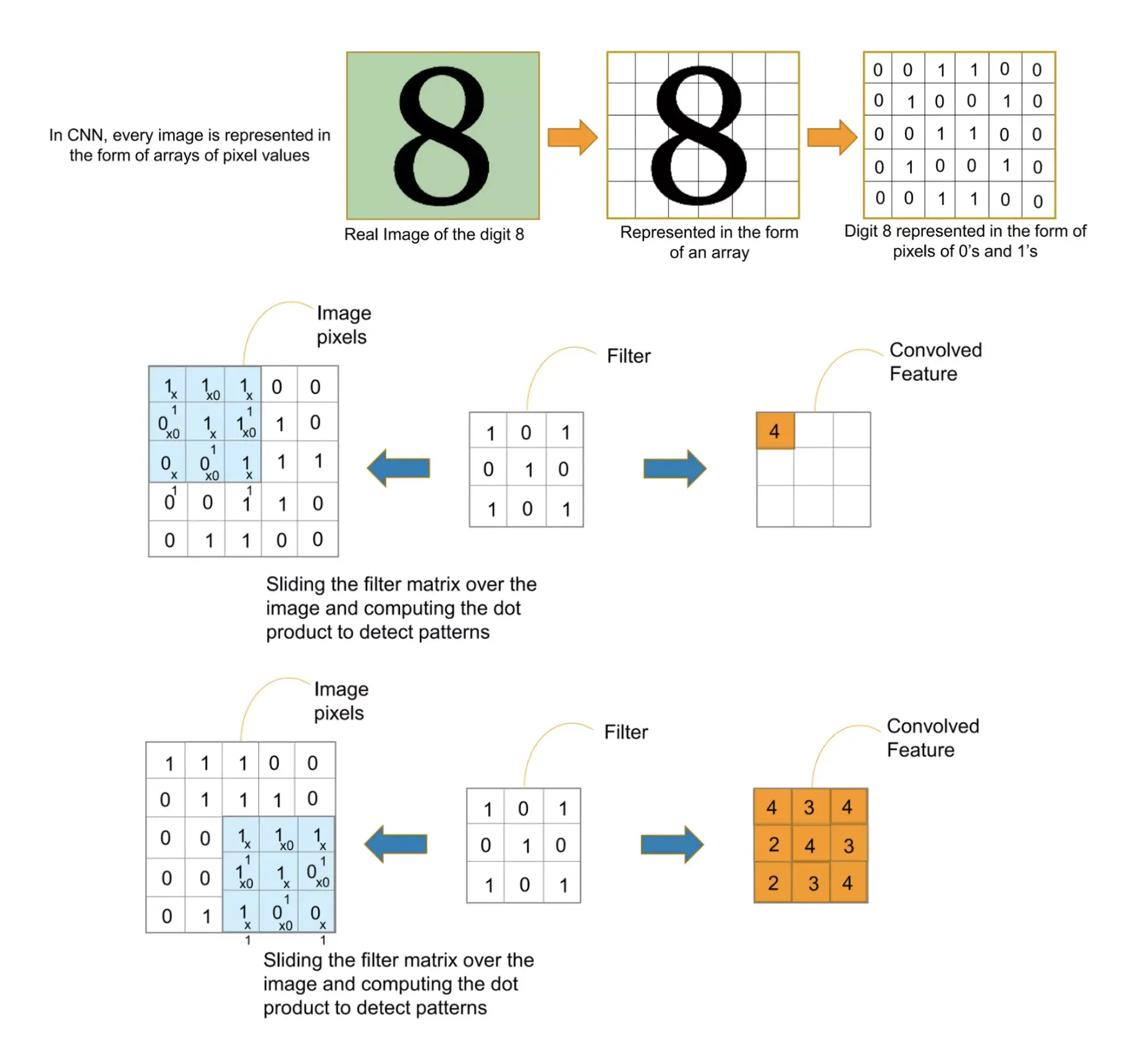
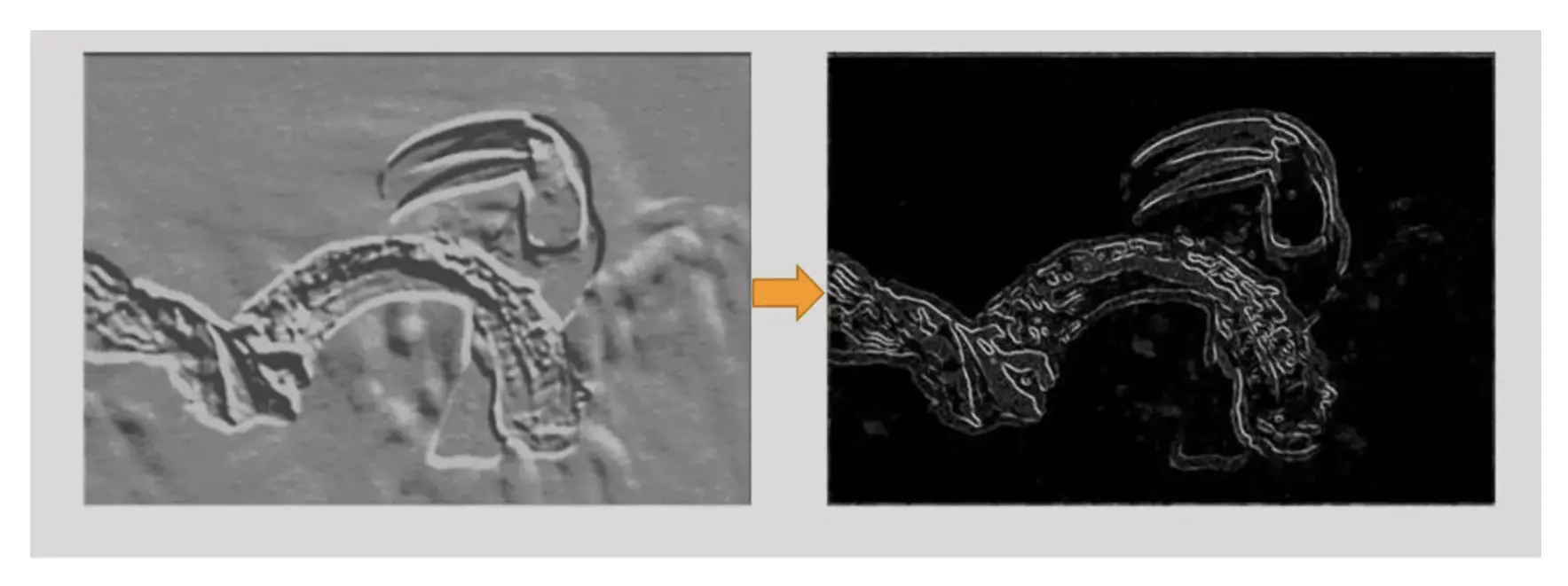
Each filter is crafted to identify specific types of features within the image, such as edges, textures, or patterns. The convolution operation employs these filters on the image, generating a feature map that emphasizes the detected features.
In the model, 32 filters, each measuring 3x3, are utilized, and ‘same’ padding is applied to ensure the output size matches the input size. Consequently, this process maintains the original input images’ size at 32x32 pixels with 3 channels (RGB).
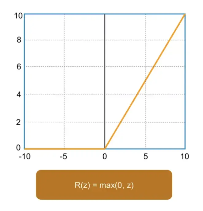
Following the convolution operation, the feature map is processed through an Activation Function. This function is essential in neural networks, as it introduces non-linearity to the network’s output. The model uses the ReLU (Rectified Linear Unit) activation function due to its ability to accelerate training while still allowing the model to converge effectively. ReLU achieves this by converting all negative values in the feature map to zero while leaving positive values as is.
Pooling Layer
Following the convolutional stages, the Pooling Layer is encountered. This layer’s main function is to diminish the spatial dimensions (width and height) of the input volume destined for subsequent convolution layers. It achieves this by summarizing the presence of features within patches of the feature map. This process aids in making the feature detection robust to changes in scale and orientation, while also lightening the computational load on the network.
There are two primary types of Pooling: Max Pooling and Average Pooling. The model uses Max Pooling, where the maximum value from each patch of the feature map is retained, and the rest are discarded. This approach contrasts with Average Pooling, which computes the average value of each patch on a feature map.
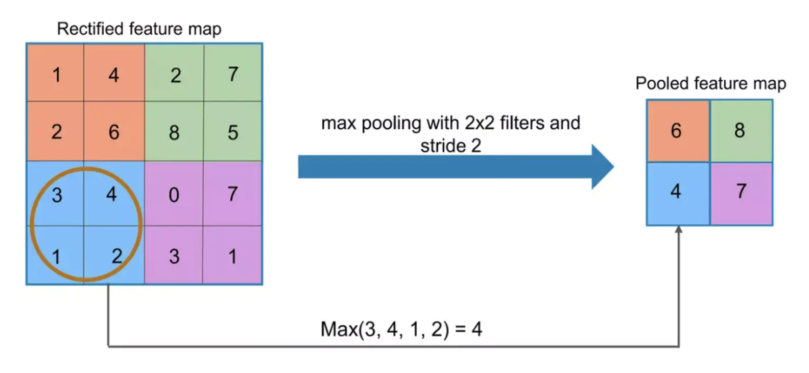
Pooling in the model is conducted over 2x2 windows with a stride of 2.
By repeatedly applying Convolutional and Pooling Layers, the network is capable of extracting increasingly complex and abstract features at each level. The initial layers may identify simple shapes or textures associated with reptiles, whereas the deeper layers are adept at recognizing entire objects or specific parts.
As the project progresses through the model, the number of filters in the Convolutional Layers is increased (from 64 to 128), enabling the network to learn more intricate features at each stage. This escalation is complemented by consistent use of ‘same’ padding and the ReLU activation function.
Fully Connected Layer
Prior to introducing the data into the fully connected layers, it must be flattened into a singular vector. This flattening process converts the complete batch of feature maps generated by the preceding layers into one elongated vector, suitable for processing by the fully connected layers. This transformation is crucial as fully connected layers require input data in a flattened vector format, as opposed to a multidimensional array.
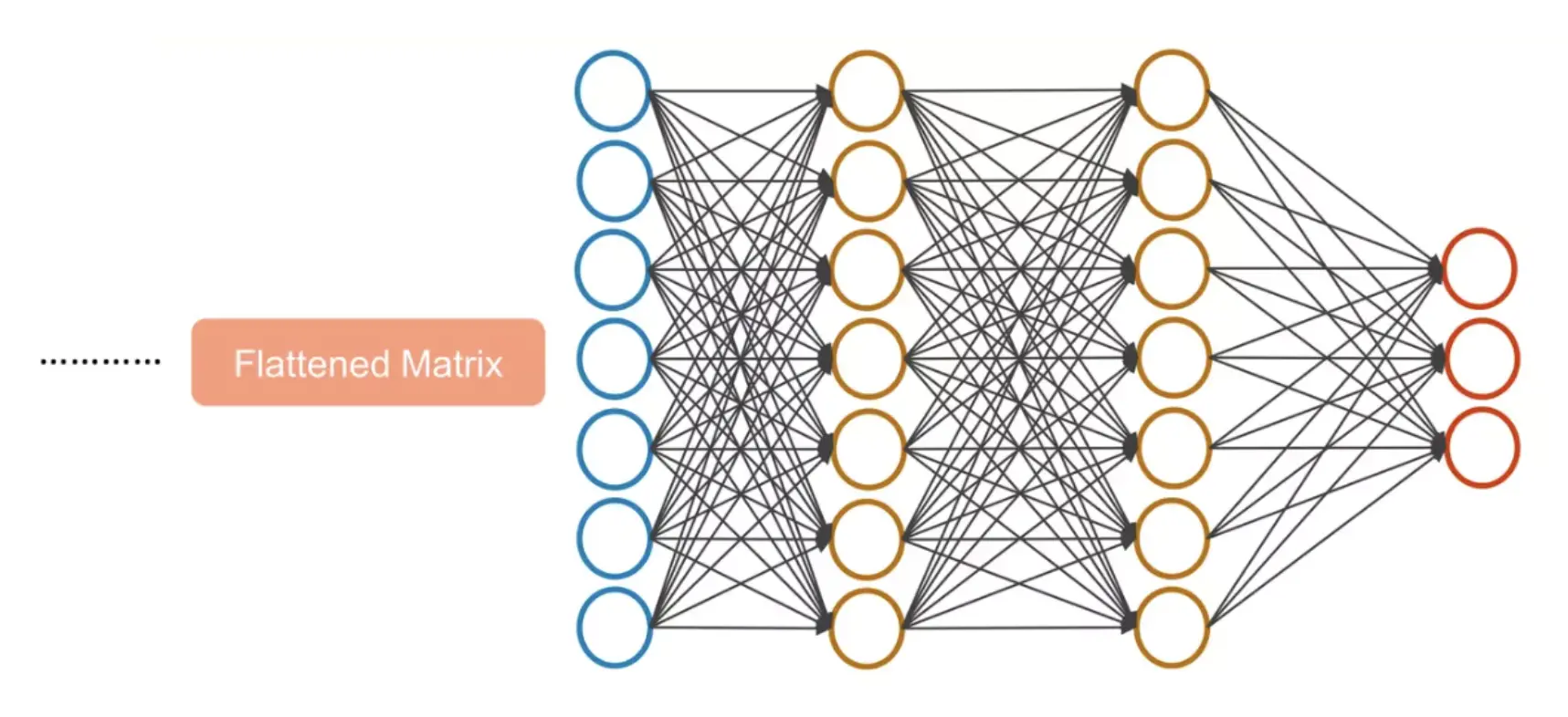
In the fully connected layer, neurons are fully connected to all activations in the previous layer, similar to what is observed in regular neural networks. Their function is to interpret the high-level filtered images (after being flattened) and convert them into votes or probabilities for various classes. This layer is crucial for the final classification decision, utilizing the complex features extracted by the convolutional and pooling layers to determine whether the image depicts a crocodile, dinosaur, lizard, snake, or turtle.
In the model, the fully connected layer is configured with 128 neurons and a ReLU activation function, which processes the flattened input to discern global patterns in the data. The final layer is another fully connected layer, this time with 5 neurons (one for each subclass within the “Reptiles” superclass), and employs the Softmax activation function to calculate probabilities for each class.
Regularization
One challenge that many machine learning models encounter, including this model, is overfitting. Overfitting occurs when a model learns the details and noise in the training data to such an extent that it adversely affects the model’s performance on new, unseen data. An overfitted model becomes overly complex, capturing spurious patterns in the training data that do not generalize well.
To combat this issue, the project implemented several key strategies.
Regularization is a technique aimed at preventing overfitting by penalizing high-valued model parameters or overly complex models, thus promoting simpler models that generalize better to new data.
The project employed Dropout, a specific regularization technique that randomly “drops out” (i.e., sets to zero) a portion of neurons in the network during each training iteration. In the model, the Dropout rate is set to 0.5, meaning 50% of the inputs are randomly zeroed during training. This approach prevents neurons from co-adapting too closely to the training data, encouraging the network to learn more robust features that generalize better. Note that during model evaluation, Dropout is not applied, allowing the network to utilize all neurons.
Additionally, the project used the EarlyStopping callback, which stops the training process if the model’s performance on a validation dataset ceases to improve. EarlyStopping’s patience was set to 5, indicating the training will halt if there’s no improvement observed for 5 consecutive epochs. This technique’s effectiveness will be highlighted in the Model Training section.
Optimization
Optimization algorithms adjust the weights of a neural network to minimize the loss function, which is a formula that measures the discrepancy between the model’s predictions and the actual target values. This minimization improves the model’s accuracy.
For the loss function, the project chose Categorical Cross Entropy, suitable for multi-class classification tasks. It measures the dissimilarity between the true label distribution and the model’s predictions. The Adam (Adaptive Moment Estimation) algorithm was selected for optimization due to its efficiency, combining elements from RMSprop and momentum to dynamically adjust the learning rate for each network weight based on the gradients’ first and second moments. This enables Adam to find an optimal set of weights more effectively than many other optimization methods.
Hyperparameter Tuning
Through extensive experimentation and trial-and-error testing, the project adjusted these hyperparameters to identify the optimal model performance for the project. This process led to selecting the following hyperparameter values:
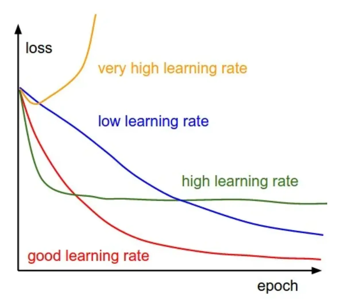
- Learning Rate: 0.001
- Batch Size: 32
- Epochs: 50
- Dropout Rate: 0.5
Augmentation
To enhance the model’s robustness, the project has integrated Data Augmentation into the Model Training process. This technique enriches the diversity of the training set by applying random, yet realistic, transformations such as rotation, shifting, and flipping.
For this model, the project implemented the following transformations along with their specific parameters:
- Rotation range: 15 degrees
- Width Shift range: 0.1 (10%)
- Height Shift range: 0.1 (10%)
- Horizontal Flip: True (enabled)
- Fill Mode: 'nearest'
Batch Size
Model Training leverages the Training and Validation Sets from the dataset, while Model Evaluation (discussed in the subsequent phase) utilizes the Test Set. Given the batch size of 32, this defines the number of batches (or iterations) performed in one epoch during Model Training, as well as the iterations during Model Evaluation. The iteration counts differ between these stages due to the varying number of images processed in each.
The formula for determining the number of batches (or iterations) is as follows:
During Model Training, which involves both the Training Set and Validation Set, the calculation of the number of batches (or iterations) per epoch exclusively utilizes the total number of images in the Training Set:
Model Evaluation
After training the model with the Training and Validation sets, the project proceeds to evaluate its performance using the Test set. This step is crucial for assessing how well the model generalizes to new, unseen data.
To visualize and better understand the model’s performance, the project plots these metrics. The project uses line graphs to compare Training and Validation losses and accuracies across multiple epochs. Additionally, the project employs a bar graph to highlight the discrepancy between Training and Validation losses at their final epoch against the Test loss, as well as to show the difference between Training and Validation accuracies at their final epoch compared to the Test accuracy.
By generating line graphs for these metrics, this yields Loss Curves and Accuracy Curves, which yield valuable insights into the model’s learning behavior.
The Loss Curve charts the changes in the loss function value throughout training. The loss function measures the discrepancy between the model’s predicted outputs and the actual target values. A descending loss curve signifies that the model is increasingly predicting more accurately over time.
The Accuracy Curve charts the model’s prediction accuracy over time, where accuracy is defined as the ratio of correct predictions to all predictions made. An ascending accuracy curve signifies that the model is learning effectively and enhancing its predictions as training progresses.
For optimal performance, particularly regarding the model’s ability to generalize to unseen data, it’s crucial for the training loss and validation loss, as well as the training accuracy and validation accuracy, to exhibit minimal divergence from each other. When training and validation losses are closely aligned, it suggests that the model is identifying patterns that extend well beyond the training dataset, indicative of strong model performance. Conversely, a pronounced discrepancy between training and validation losses, particularly when validation loss is significantly higher, points to overfitting. This condition implies that the model might be memorizing the training data instead of learning to generalize.
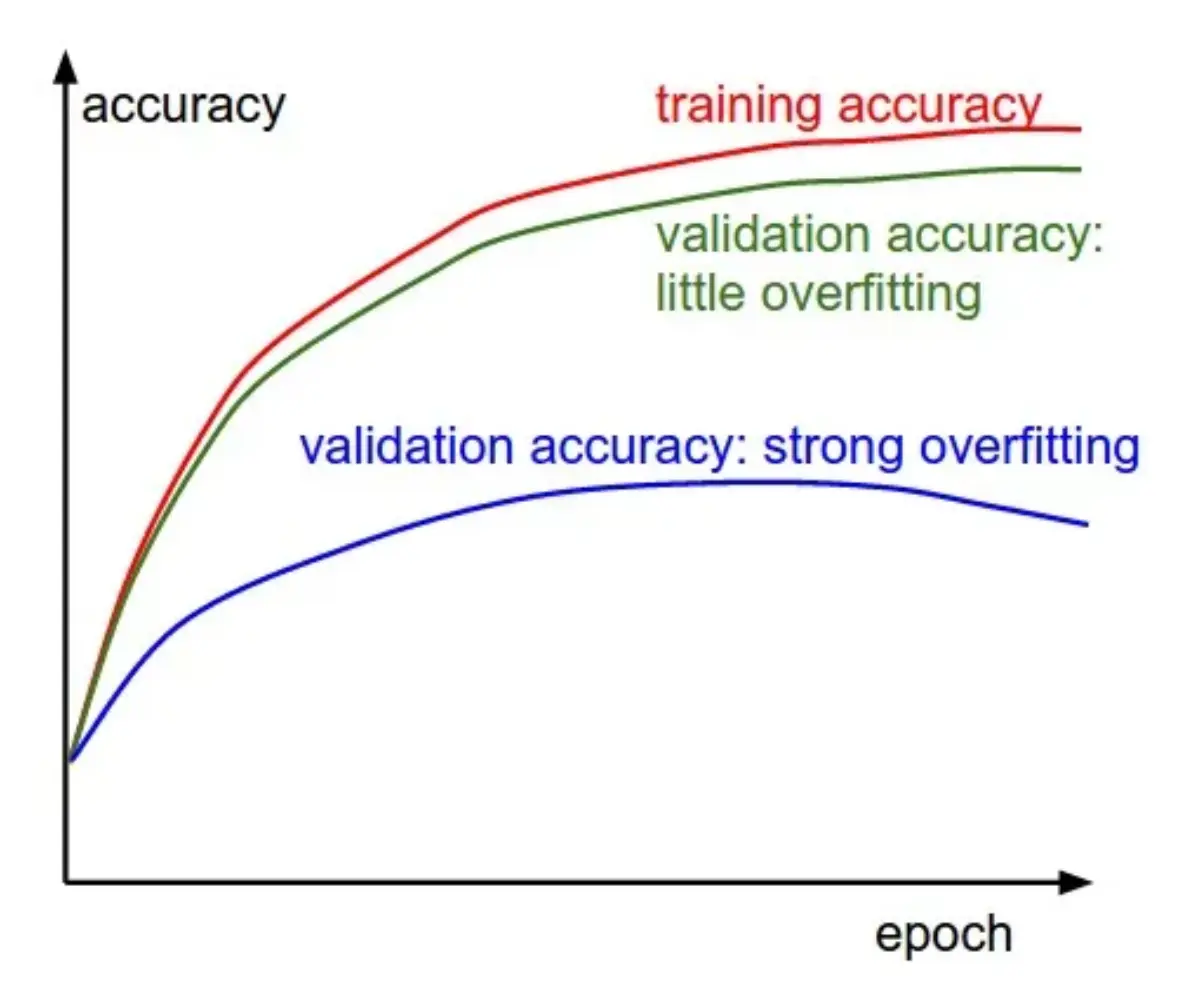
Similarly, when training and validation accuracies are nearly equivalent, it denotes that the model performs equally well on unseen data as on the training set, highlighting effective generalization. A notable gap between training accuracy and validation accuracy suggests overfitting, indicating the model’s tendency to memorize rather than learn from the training data.
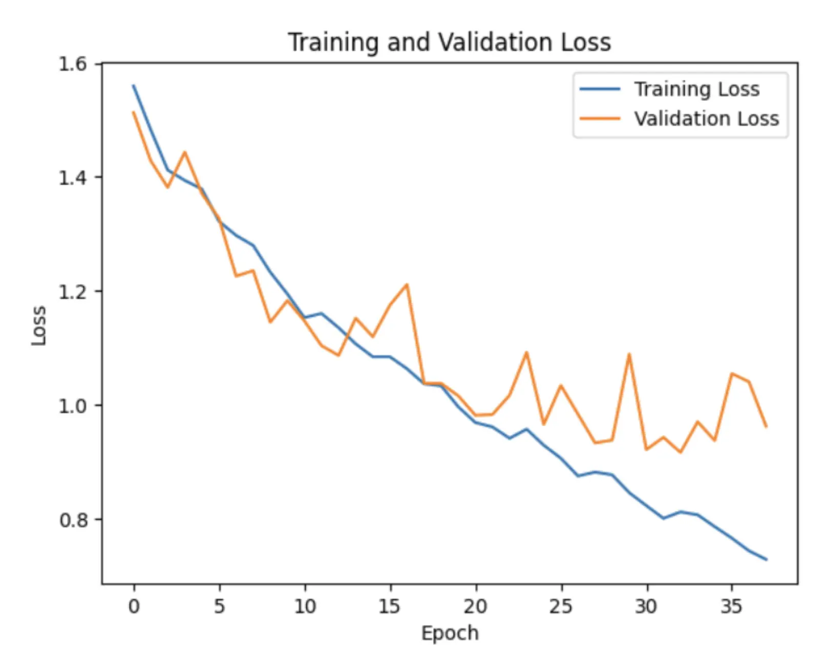
The Training and Validation Losses showcase decreasing loss curves. This trend indicates that the model is learning to predict more accurately over time. Furthermore, the proximity of the training and validation losses, with minimal divergence, suggests that the model is effectively learning patterns that generalize beyond the training dataset, thereby indicating strong model performance.
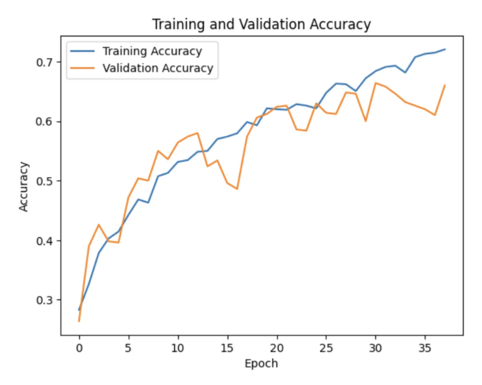
The Training and Validation Accuracies reveal ascending accuracy curves. This indicates that the model is learning effectively, with its predictions becoming more accurate over time. Additionally, the closeness of the training and validation accuracies, marked by a minimal gap, suggests that the model performs equally well on unseen data as it does on the training data, indicative of good generalization.
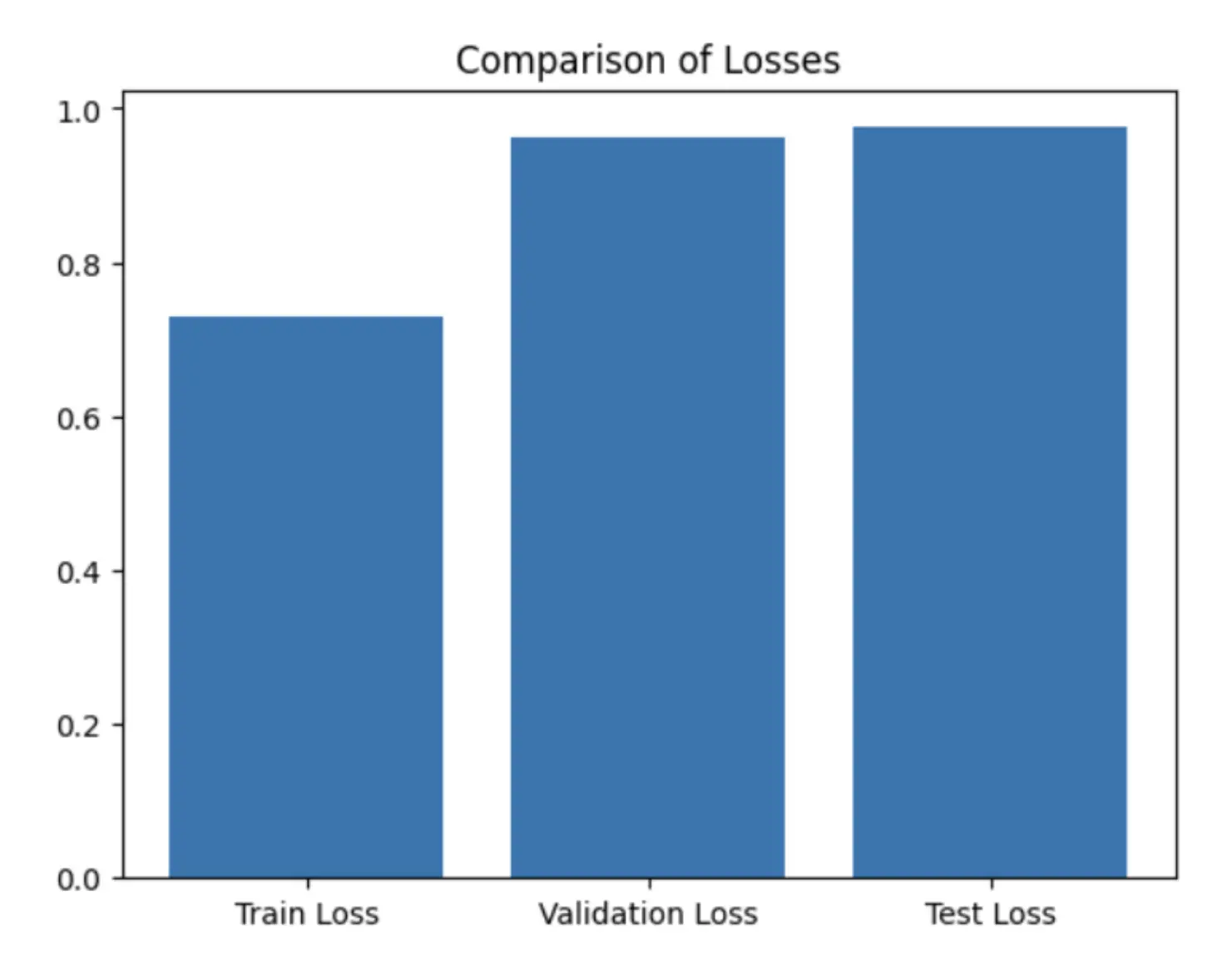
Comparing the Training, Validation, and Test Losses, as anticipated, the training loss is the lowest, reflecting the model’s direct training to minimize this value. The validation loss is marginally higher than the training loss, a typical outcome since the validation set serves to evaluate model performance on unseen data during training. The test loss registers as the highest, suggesting the model’s performance on the test set is slightly inferior compared to the training and validation sets. However, the disparities are not significant, suggesting that the model is generalizing fairly well.
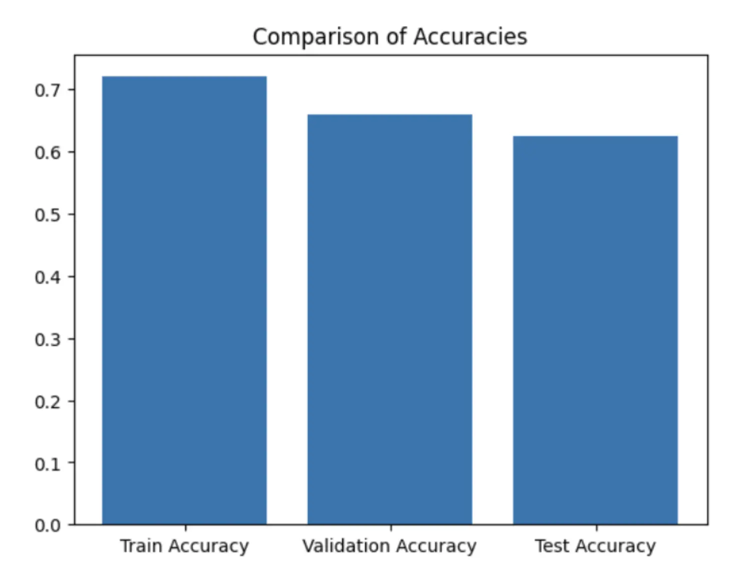
Comparing the Training, Validation, and Test Accuracies, the training accuracy is the highest, indicating that the model performs optimally on the data it has been trained on. The validation accuracy is marginally lower than the training accuracy, a common observation that demonstrates the model’s capacity to generalize to new, unseen data. The test accuracy is subtly lower than the validation accuracy but remains closely aligned with the training accuracy, which again suggests a good level of generalization.
In summary, the proximity of the test loss to the validation and training losses, along with the test accuracy being close to the validation and training accuracies, suggests that the model generalizes effectively to unseen data. There’s no evident overfitting. Typically, overfitting is marked by a low training loss with significantly higher validation and test losses, or high training accuracy with considerably lower validation and test accuracies. Moreover, the consistency of losses and accuracies across the three datasets (training, validation, test) is a promising indicator that the model is not merely memorizing the training data but is learning patterns that are broadly applicable. This balance between learning from the training data and performing well on unseen data aligns with the objectives of a well-adjusted model. Nonetheless, the presence of a gap between training and test losses, albeit not substantial, indicates there may still be opportunities for enhancement, as the model has not achieved flawless accuracy.