By John Ivan Diaz
A simple desktop application that predicts the next path of a typhoon based on observed data points of its previous trajectory. Python and PyQt were used for full-stack development. Although the forecasting is limited to historical path data and does not account for other factors influencing a typhoon’s movement, the application is primarily designed to illustrate the concepts of interpolation and extrapolation.
Discovery Phase
Tropical cyclones, formidable storm systems characterized by low pressure, intense winds, and heavy rainfall, are intricately tied to the Earth’s geographical features. The planet’s latitude and longitude lines define the specific locations where tropical cyclones form, with warm ocean waters serving as their incubators. Earth’s division into the Northern and Southern Hemispheres plays a crucial role in the behavior of these storms, as the Coriolis effect influences wind directions differently in each hemisphere. This hemispheric distinction is pivotal when discussing tropical cyclones, as it determines their rotation and trajectory. In the Northern Hemisphere, these storms are known as typhoons or hurricanes, while in the Southern Hemisphere, they are referred to simply as cyclones. This nomenclatural variation reflects the importance of understanding the hemispheric context in comprehending the development and movement of these powerful meteorological phenomena.
This project involves a simulation for mapping the trajectory of tropical cyclones. Its goal is to monitor the changes in longitude and latitude distances of a tropical cyclone over time, from the past to the future. The program gathers historical speed data of the cyclone at specific times and smartly predicts speeds between and beyond the given data points using interpolation and extrapolation techniques. By combining this speed information with predefined time intervals, the program calculates distances traveled, providing insights into the cyclone’s position in terms of both longitude and latitude. The results are then visually presented on a graph, offering users a clear understanding of the cyclone’s movement.
Development Phase
Features
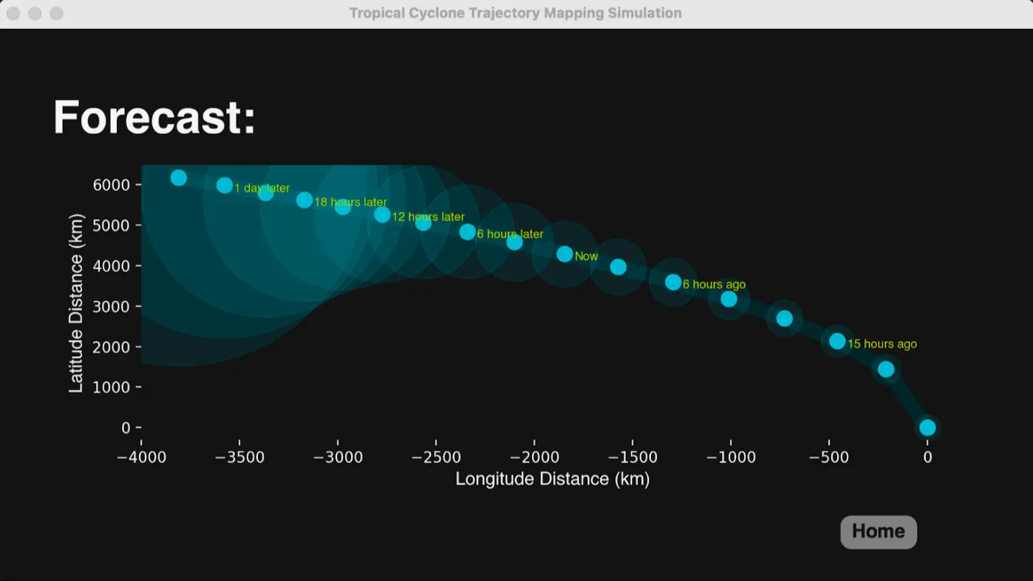
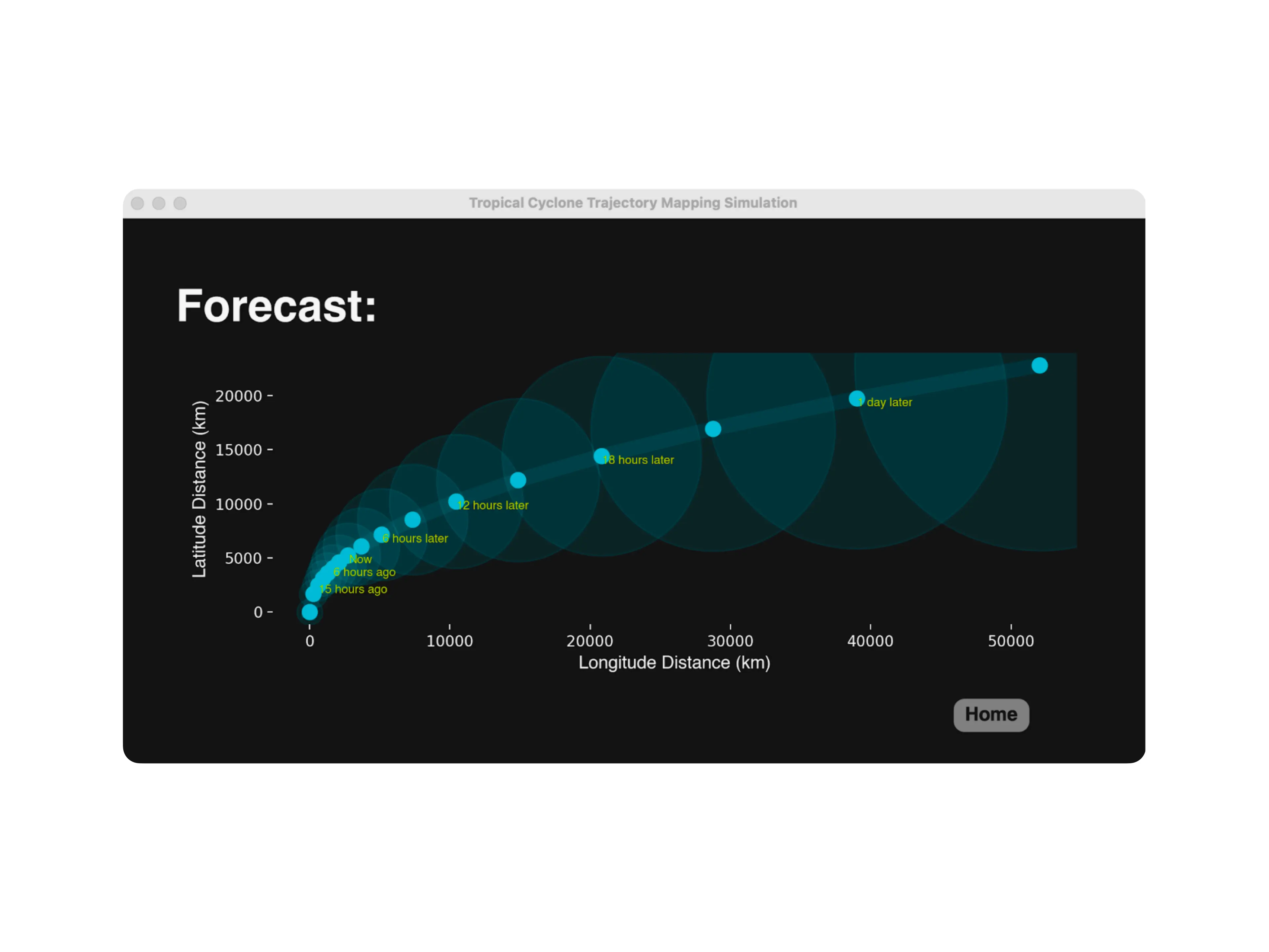
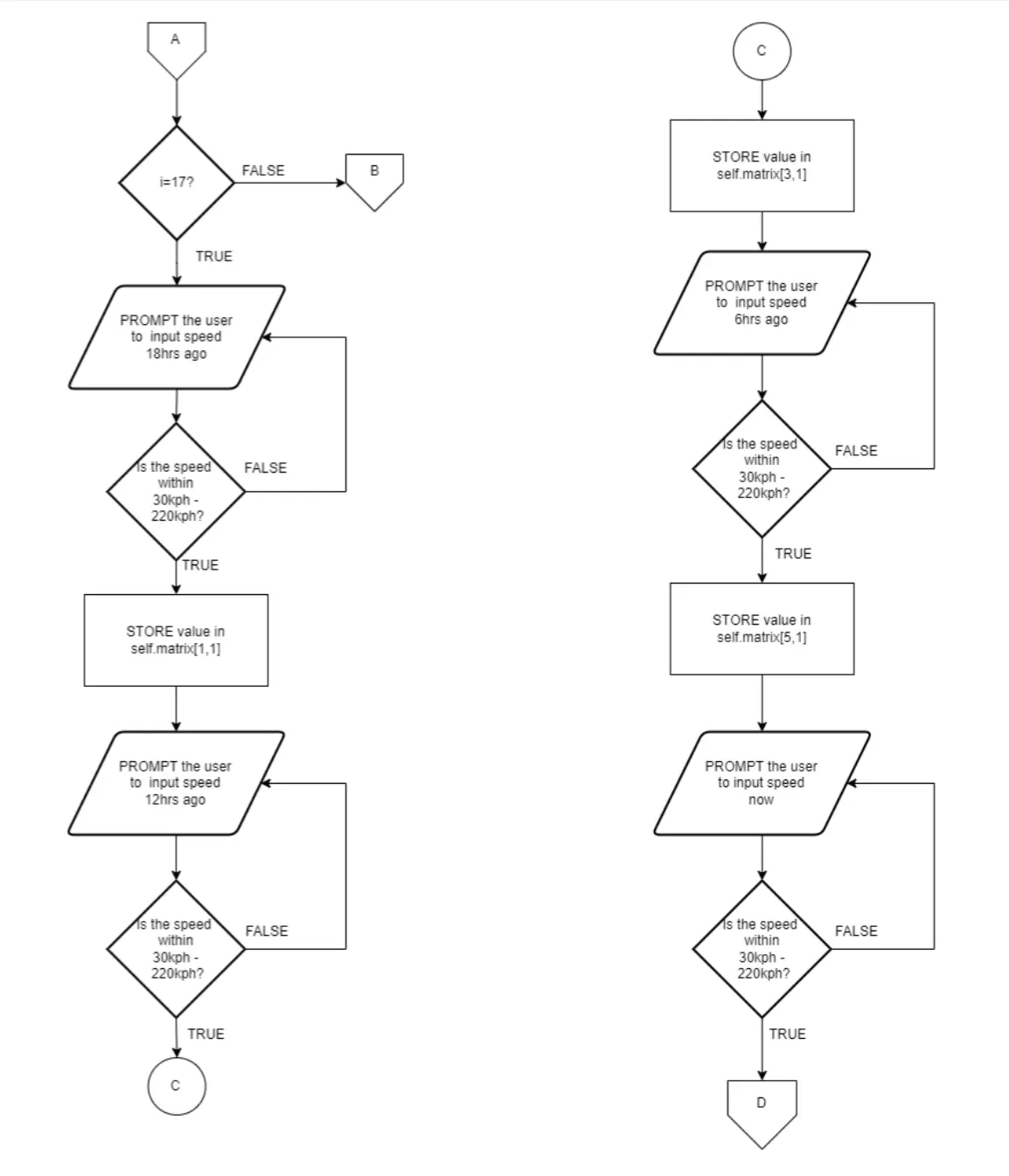
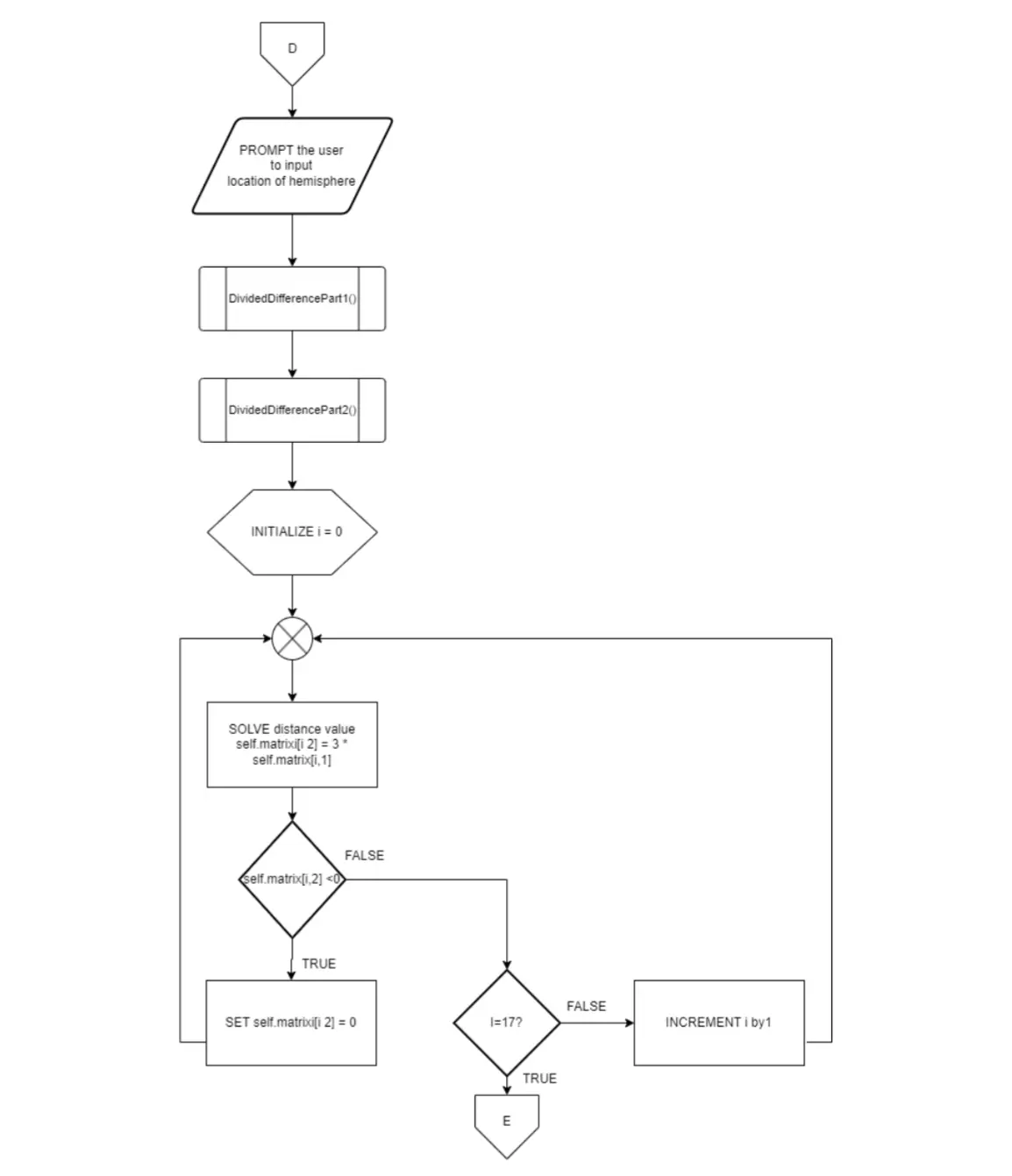
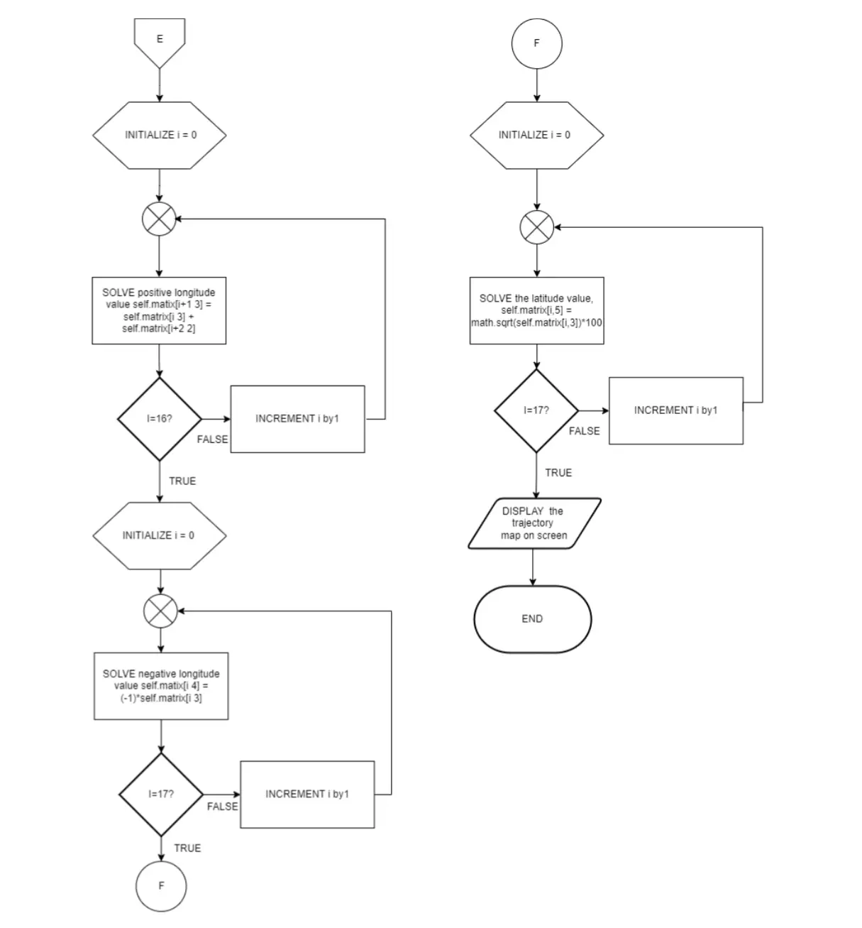
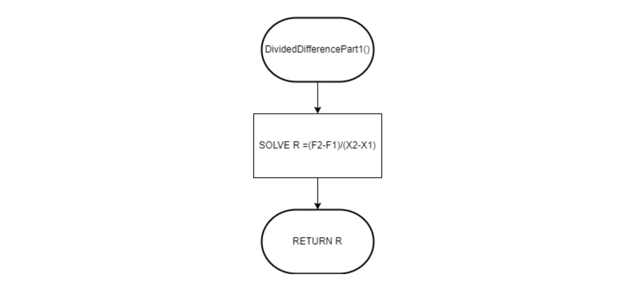
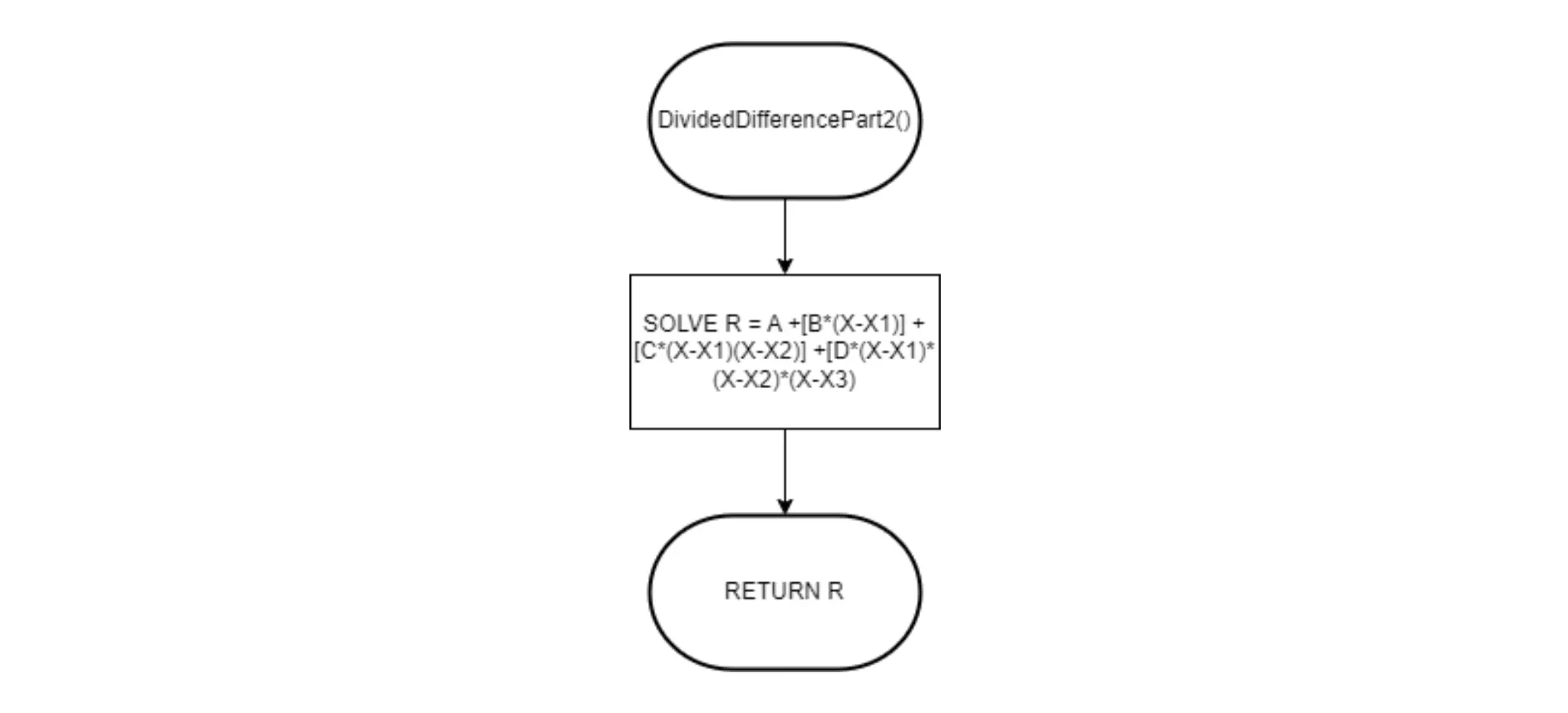
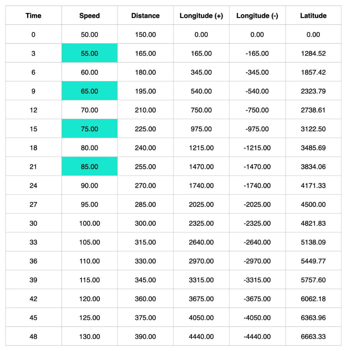
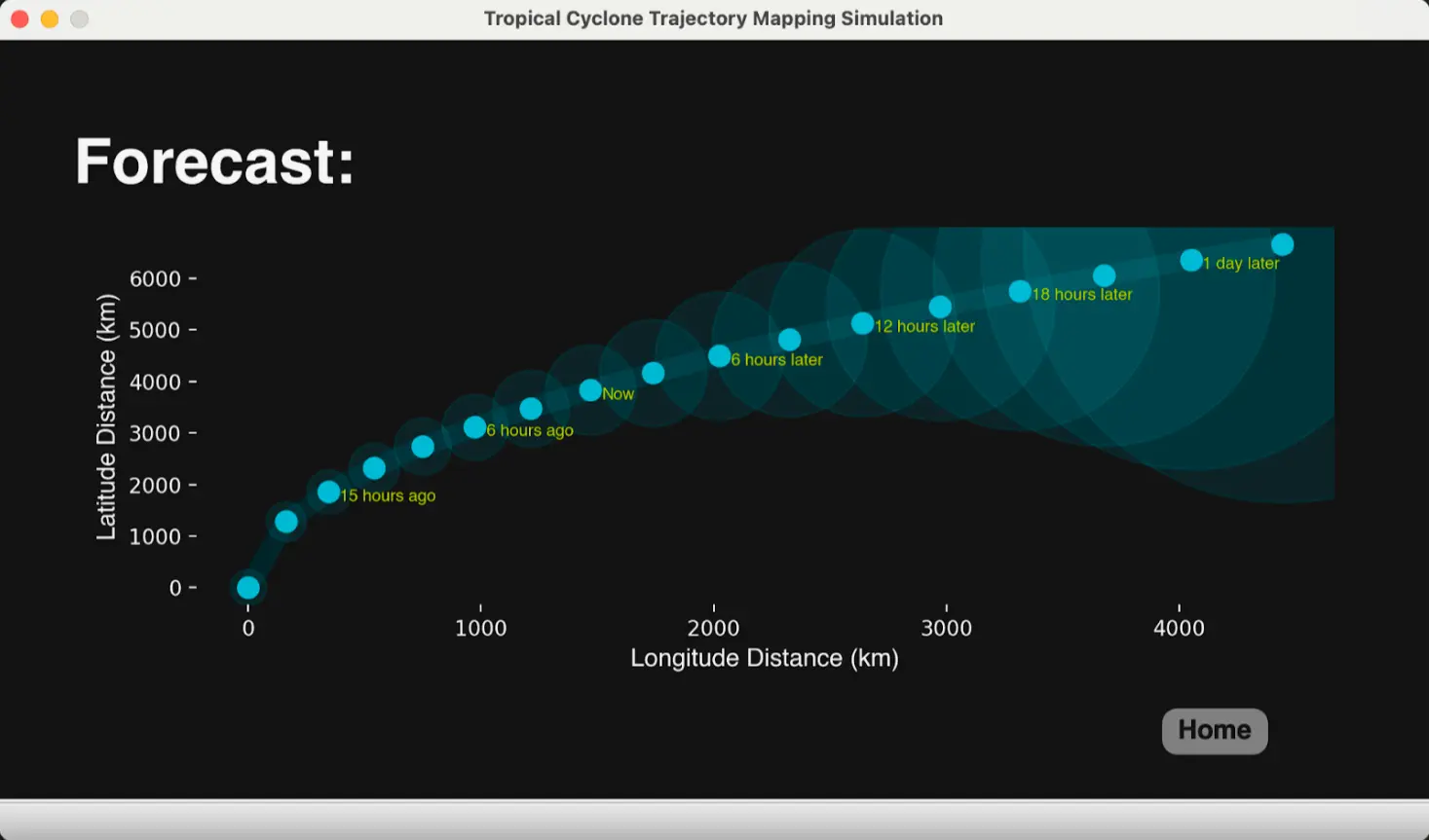
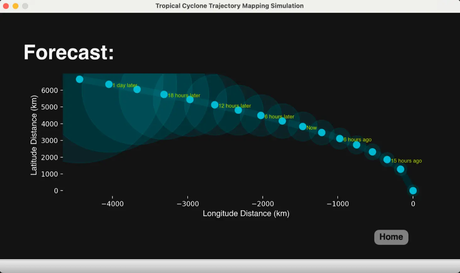
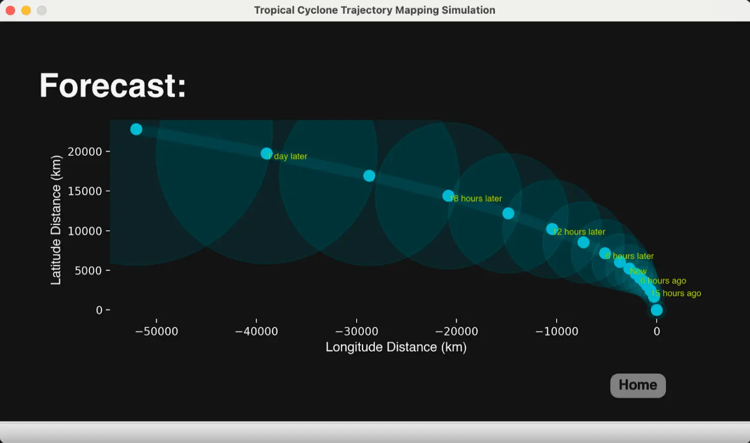
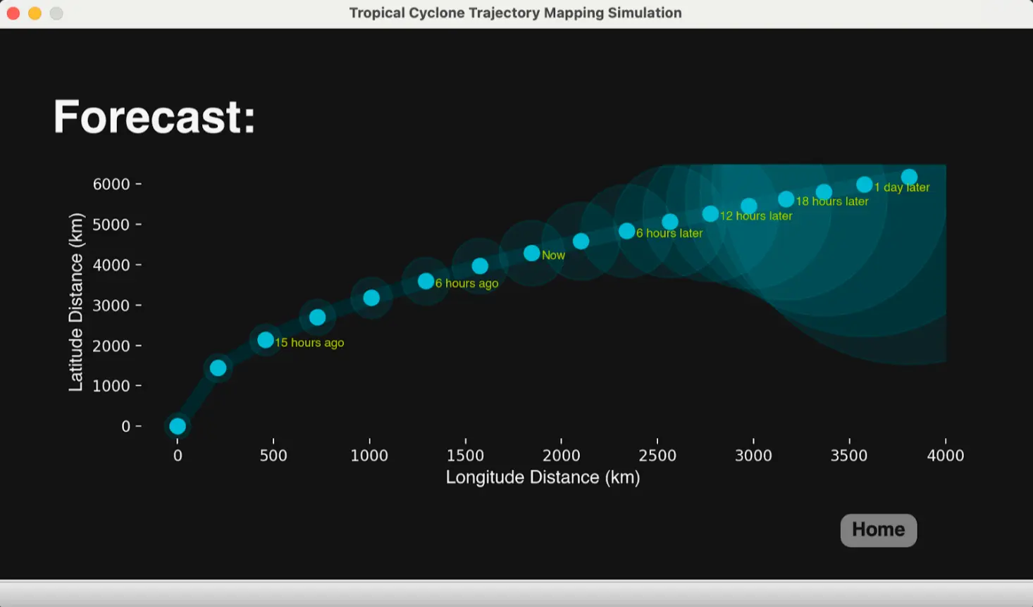
The program can map the historical and future trajectory of a tropical cyclone in terms of both longitude and latitude. It first collects speed data at intervals: 18 hours ago, 12 hours ago, 6 hours ago, and the current speed. To fill in the gaps between and beyond these timestamps (where speeds are unknown), the program employs interpolation (for in-between data) and extrapolation (for data outside the provided timestamps) using the divided difference method at 3-hour intervals. It calculates distance by multiplying speed and a fixed time value of 3 hours. From the distance data, the program determines longitude and latitude metrics. The results are then displayed graphically, with labels indicating specific time points like 3 hours ago or 1 day later. The user can hover the cursor over the graph to track and view precise longitude and latitude values, providing an interactive way to interpret the typhoon’s accurate position at different times.
Limitations
The application doesn’t display precise Earth coordinates of the tropical cyclone’s current location and direction. Instead of mapping the trajectory on a real-world map, it simply offers insights into the cyclone’s distance over time in terms of longitude and latitude. The simulation also doesn’t consider certain real-world factors, like the presence of other nearby cyclones or the potential for landfall, making the focus on the cyclone’s general movement rather than accounting for specific conditions.
Input
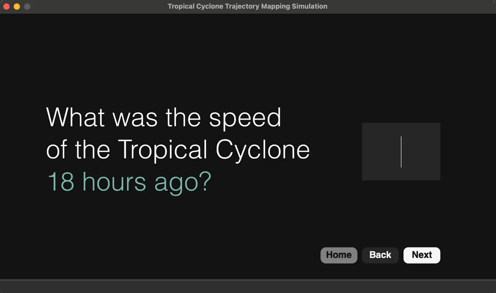
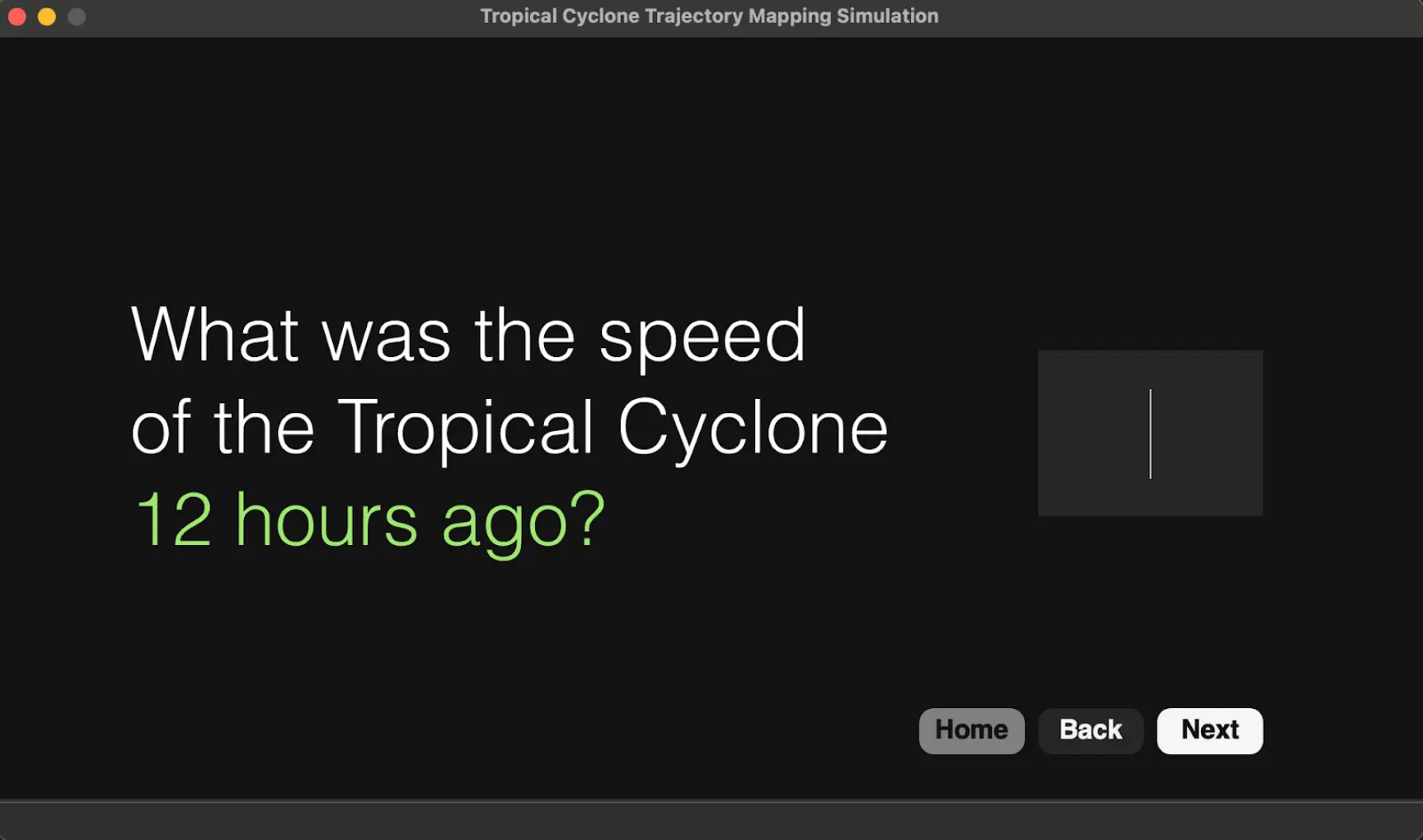
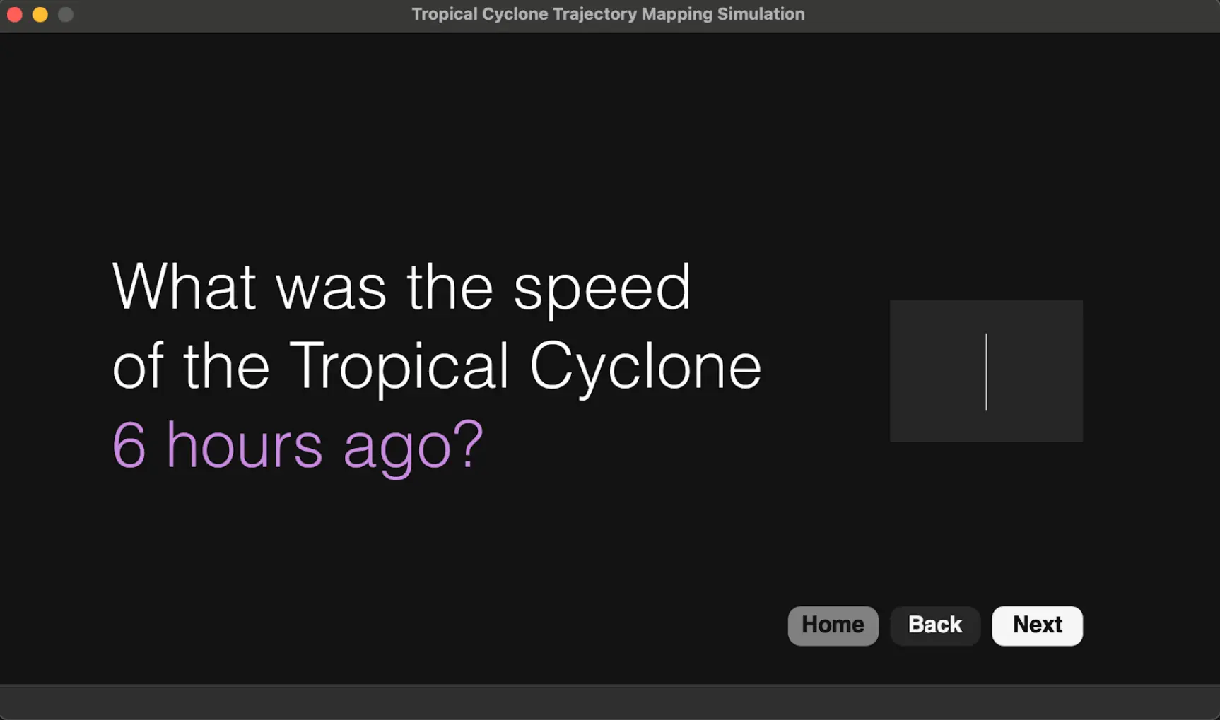
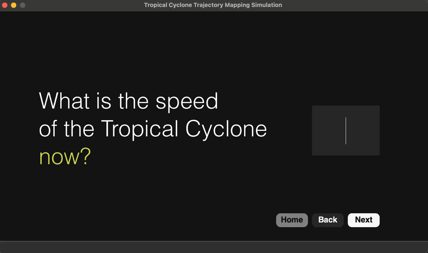
The program involves the acquisition of crucial inputs through a user prompt-driven system. The program solicits specific information related to a tropical cyclone, focusing on two key parameters:
- Tropical Cyclone Speed:
Speed readings are gathered at distinct time intervals: 18 hours ago, 12 hours ago, 6 hours ago, and the present moment (Now).
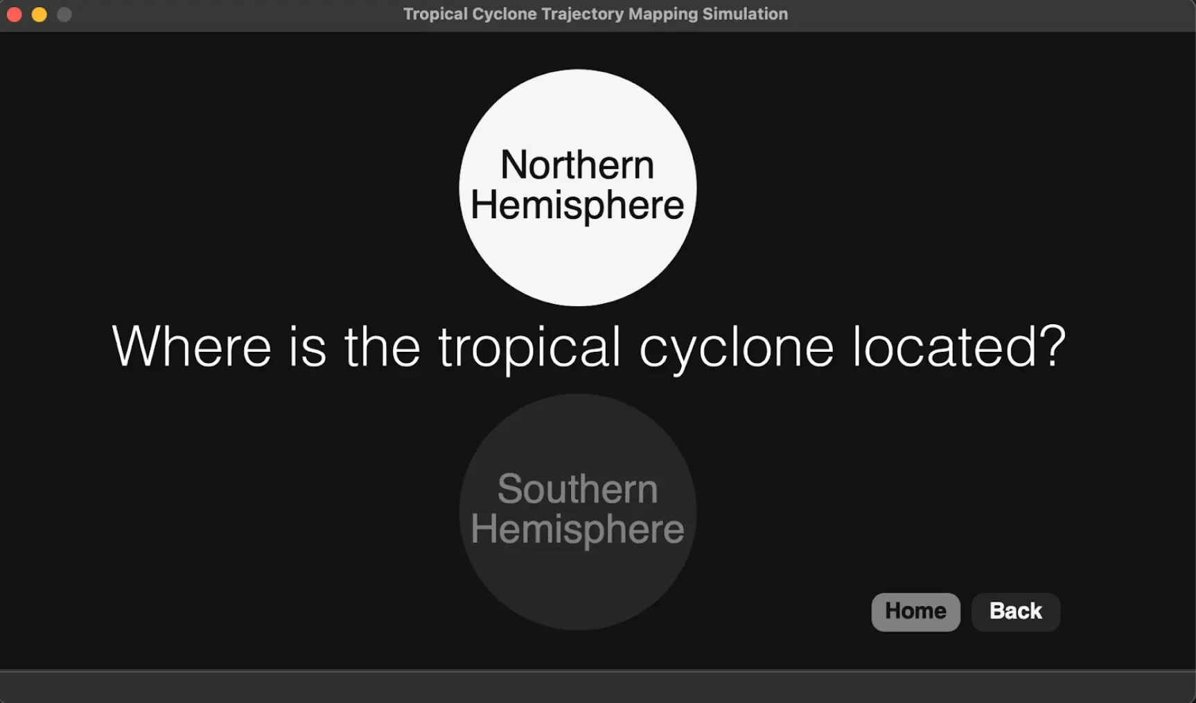
- Hemisphere Location:
Users are prompted to specify the hemisphere in which the tropical cyclone is situated, providing options for either the Northern or Southern Hemisphere.
This aims to enhance the understanding of tropical cyclone dynamics, facilitating comprehensive analyses of speed variations and their correlation with specific hemispheric locations over time.
Output
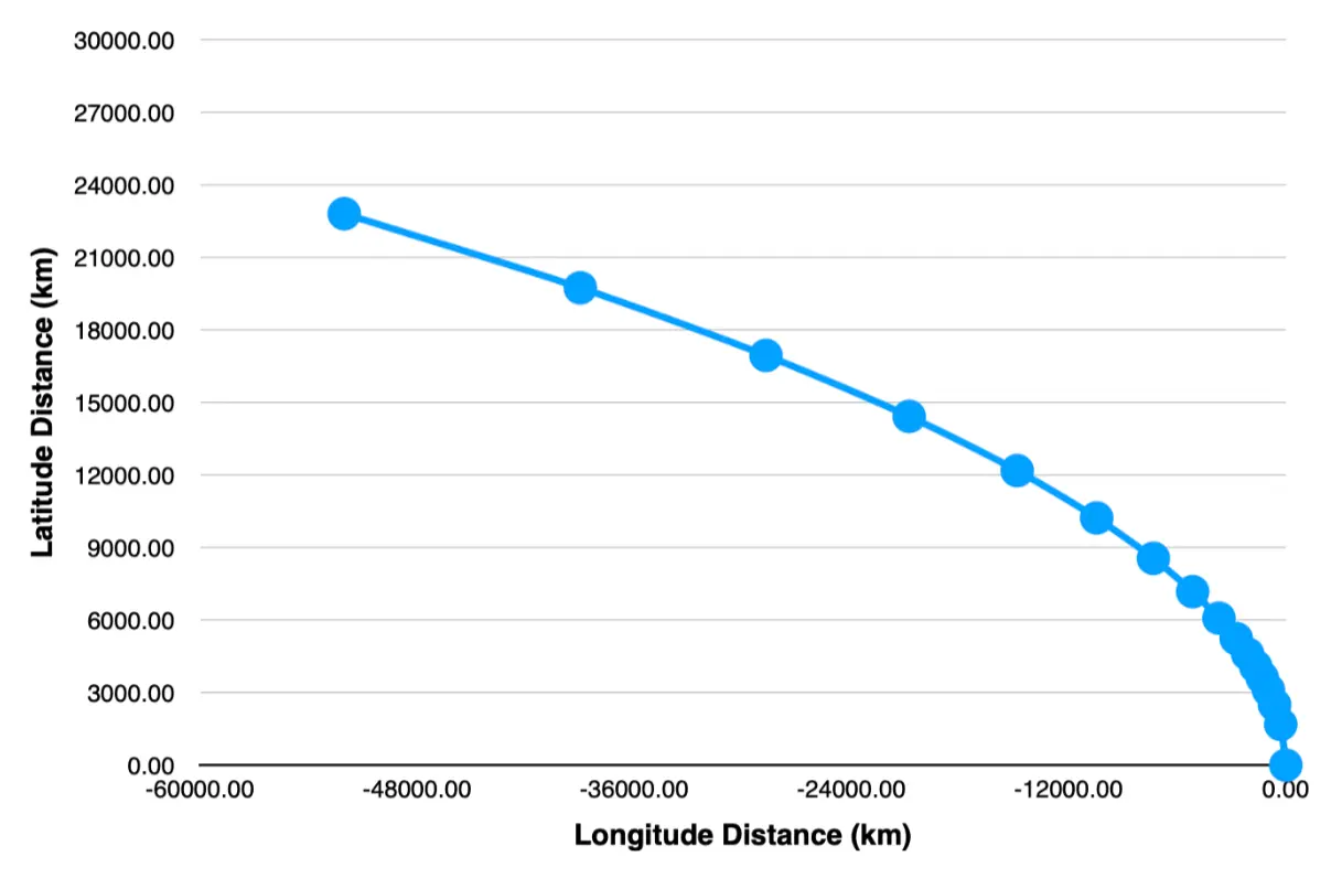
The program generates a graphical representation that conveys valuable insights to the users, comprising:
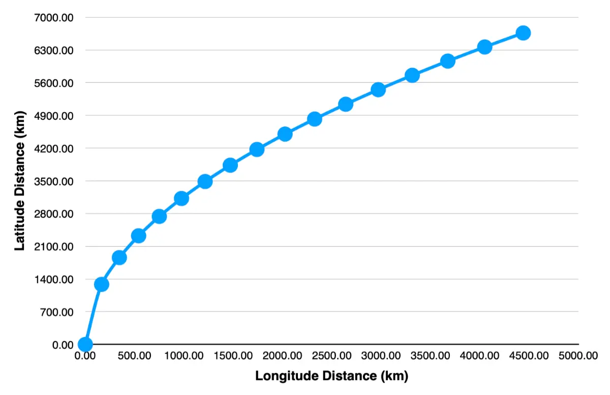
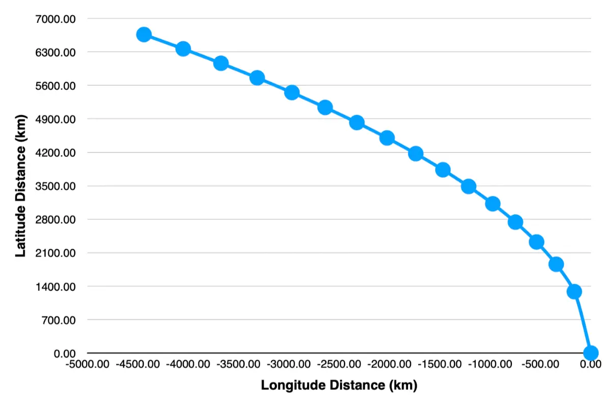
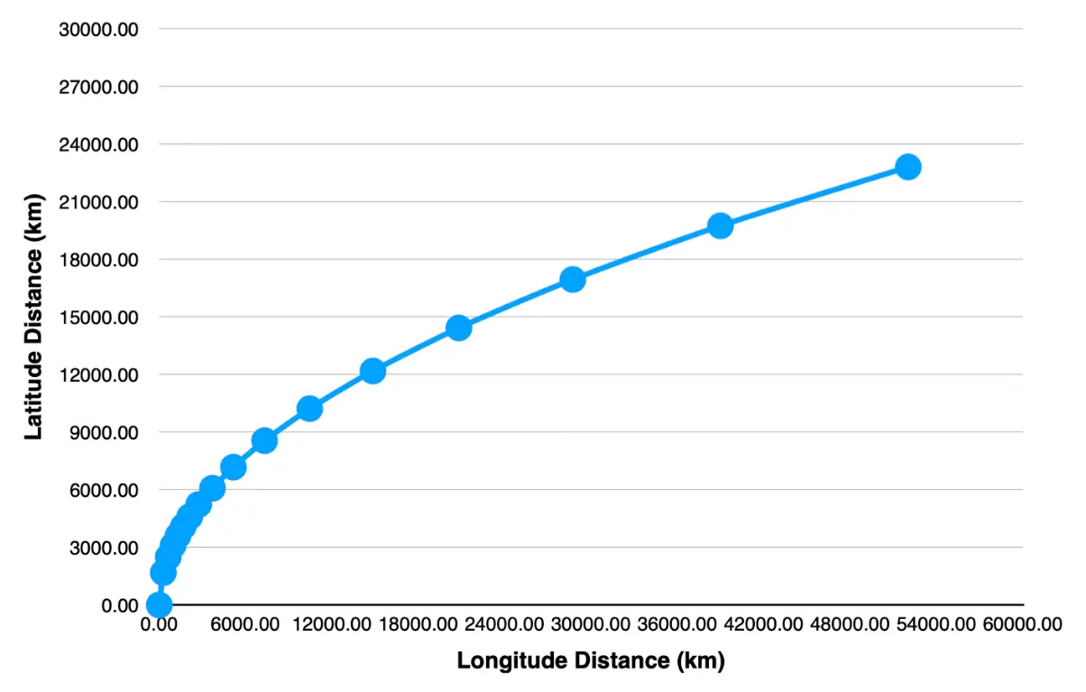
- Longitudinal distance of the tropical cyclone over time, including past occurrences, the current moment, and future projections at 3-hour intervals.
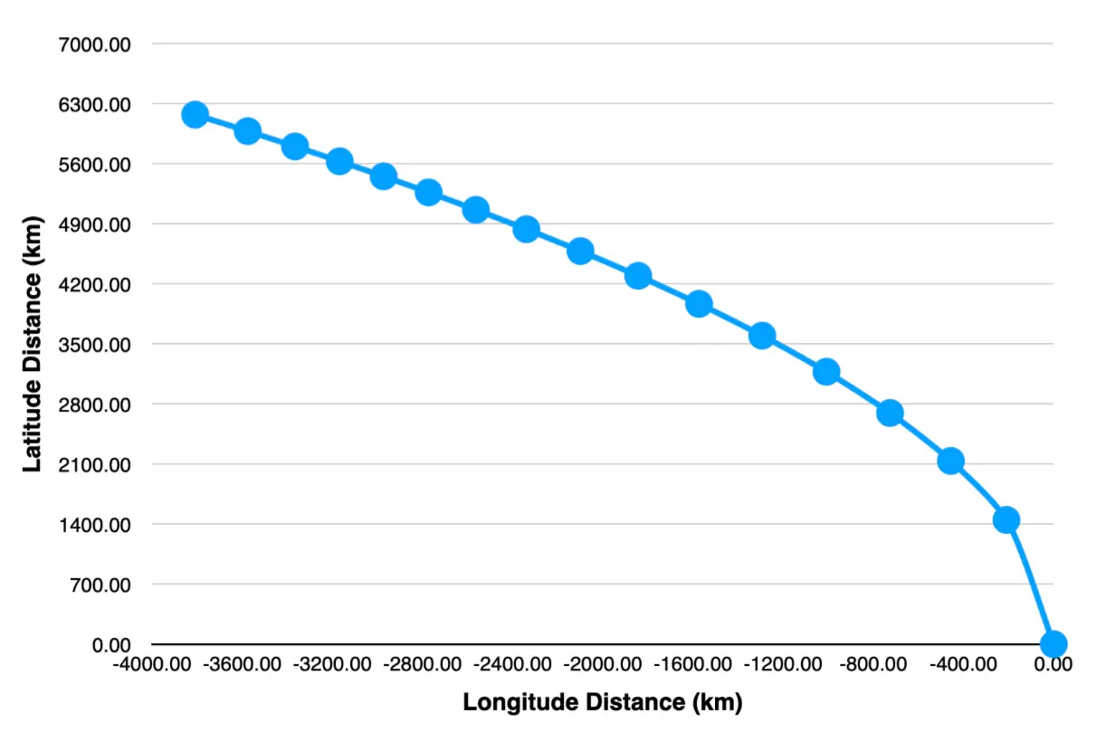
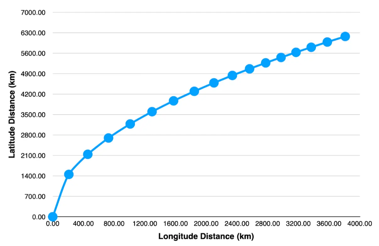
- Latitudinal distance of the tropical cyclone over time, including past occurrences, the current moment, and future projections at 3-hour intervals.
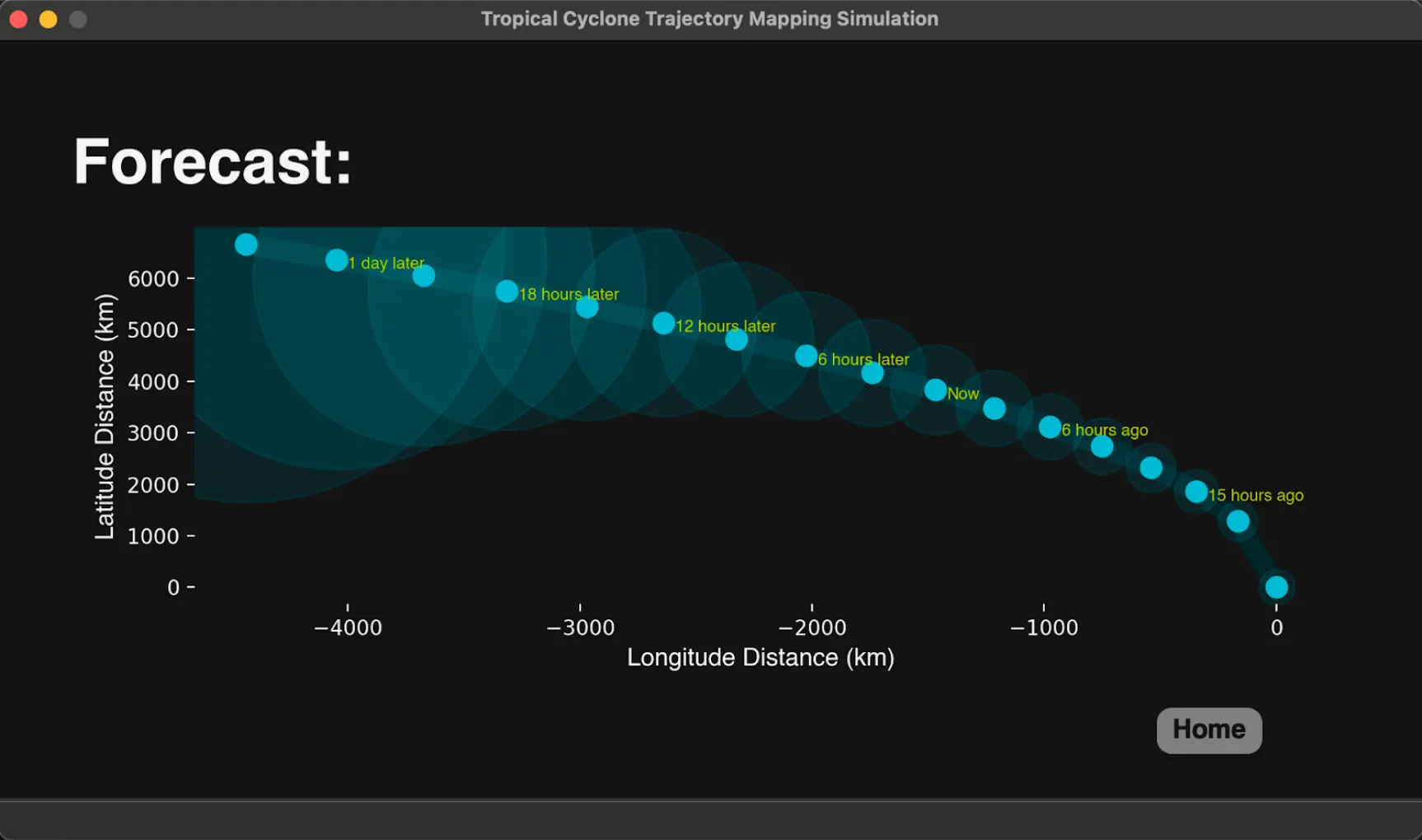
The graphical representation provides a comprehensive overview, allowing for a nuanced examination of the tropical cyclone’s distance behavior in both longitudinal and latitudinal dimensions over time.
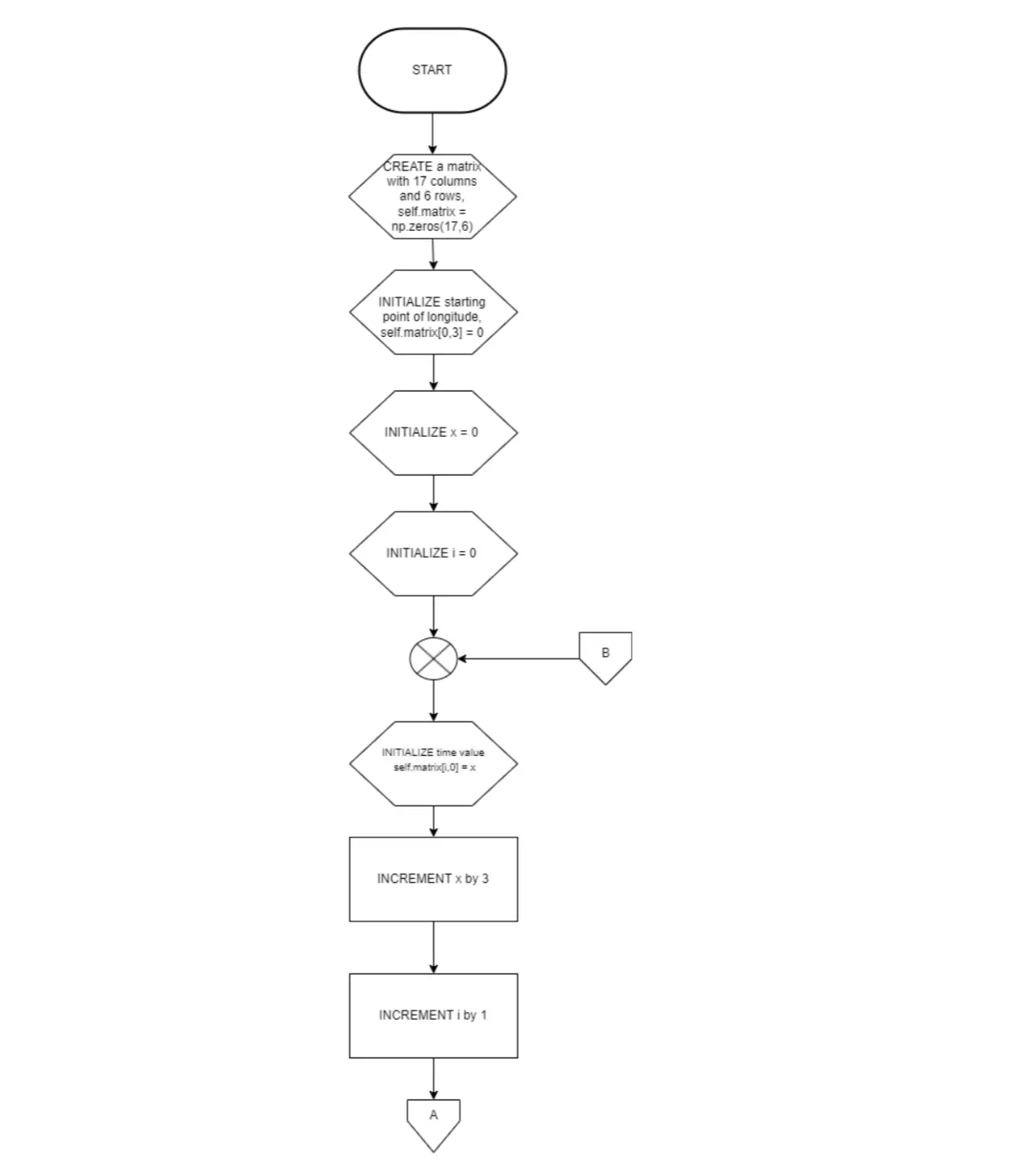
Algorithm
- Main function
- DividedDifferencePart1 function
- DividedDifferencePart2 function
Sample Input-Output
Overview of where inputs are requested and where interpolation and extrapolation are carried out:

Scenario 1:
- Speed at 18 hours ago: 55 km
- Speed at 12 hours ago: 65 km
- Speed at 6 hours ago: 75 km
- Speed at present moment: 85 km
- Hemisphere location: Southern hemisphere
- Hemisphere location: Northern hemisphere
Scenario 2:
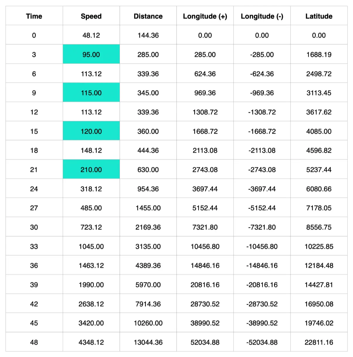
- Speed at 18 hours ago: 95 km
- Speed at 12 hours ago: 115 km
- Speed at 6 hours ago: 120 km
- Speed at present moment: 210 km
- Hemisphere location: Southern hemisphere
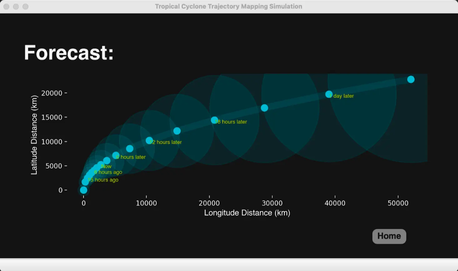
- Hemisphere location: Northern hemisphere
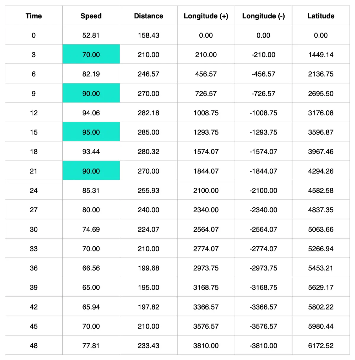
Scenario 3:
- Speed at 18 hours ago: 70 km
- Speed at 12 hours ago: 90 km
- Speed at 6 hours ago: 95 km
- Speed at present moment: 90 km
- Hemisphere location: Southern hemisphere
- Hemisphere location: Northern hemisphere